Skip to content
Free Excel Tutorials
  • Home
  • Excel For Beginners
  • Excel Intermediate
  • Advanced Excel For Experts

Data Analysis

  • Conditional Formatting Icon Sets Examples in Excel
  • Filter Data Based on Date in Excel
  • How to do a t-Test in Excel?
  • Excel Line Chart
  • Understanding Anova in Excel

References

  • Complete List of Excel Lookup and Reference Functions, References and Examples
  • Count unique text values with criteria
  • How to use Excel INDIRECT Function
  • How to calculate two-way lookup VLOOKUP in Excel Table
  • How to use Excel OFFSET function

Data Validations

  • Excel Data validation must contain specific text
  • Excel Data validation date in specific year
  • Excel Data validation allow uppercase only
  • Excel Data validation require unique number
  • Excel Data validation specific characters only

Remove last characters from right in a cell in Excel

by

To remove the last n characters from a text string, you can use a formula based on the LEFT and LEN functions. You can use a formula like this to strip the last 3 characters, last 5 characters of a value, starting on the left.

Formula

=LEFT(text,LEN(text)-n)

Note: there is no reason to use the VALUE function if you don’t need a numeric result.

Explanation

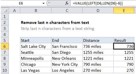
In the example shown, the formula in E6 is:

=VALUE(LEFT(D6,LEN(D6)-6))

Which trims ” miles” from each value returning just the number.

How this formula works

The LEFT function is perfect for extracting characters from the left side of a value. We use LEFT in this formula to extract all characters up to the number of characters we want to trim.

The challenge, for values with variable length, is that we don’t know exactly how many characters to extract. That’s where the LEN function is used.

Working from the inside out, LEN calculates the total length of each value. For D6 (736 miles) the total length is 9.

To get the number of characters to extract, we subtract 6, which the length of ” miles” including the space character. The result is 3, which is fed to LEFT as the number of characters to extract. LEFT then returns the text “736” as a text value.

Finally, because we want a numeric value (not text) we run the text through the VALUE function, which converts numbers in text format to plain numbers.

The formula evaluation goes like this:

=VALUE(LEFT(D6,LEN(D6)-6))
=VALUE(LEFT(D6,9-6))
=VALUE(LEFT(D6,3))
=VALUE("736")
=736

Post navigation

Next Post:

Create One-dimensional and Two-dimensional Array

Leave a Reply Cancel reply

Your email address will not be published. Required fields are marked *

Learn Basic Excel

Ribbon
Workbook
Worksheets
Format Cells
Find & Select
Sort & Filter
Templates
Print
Share
Protect
Keyboard Shortcuts

Categories

  • Charts
  • Data Analysis
  • Data Validation
  • Excel Functions
    • Cube Functions
    • Database Functions
    • Date and Time Functions
    • Engineering Functions
    • Financial Functions
    • Information Functions
    • Logical Functions
    • Lookup and Reference Functions
    • Math and Trig Functions
    • Statistical Functions
    • Text Functions
    • Web Functions
  • Excel VBA
  • Excel Video Tutorials
  • Formatting
  • Grouping
  • Others

Logical Functions

  • SWITCH function example in Excel
  • How to use Excel AND Function
  • How to use Excel NOT Function
  • Complete List of Excel Logical Functions, References and Examples
  • How to use Excel TRUE Function

Date Time

  • DAY function: Description, Usage, Syntax, Examples and Explanation
  • Convert Excel time to decimal minutes
  • Sum through n months in Excel
  • How to calculate project start date based on end date in Excel
  • SECOND function: Description, Usage, Syntax, Examples and Explanation

Grouping

  • Group times into 3 hour buckets in Excel
  • Map inputs to arbitrary values in Excel
  • Group numbers at uneven intervals in Excel
  • Map text to numbers in Excel
  • Group times into unequal buckets in Excel

General

  • How to generate random times at specific intervals in Excel
  • Currency vs Accounting Format in Excel
  • Find, Trace and Correct Errors in Excel Formulas using ‘Formula Auditing’
  • Cell References: Relative, Absolute and Mixed Referencing Examples
  • Convert column number to letter in Excel
© 2025 xlsoffice . All Right Reserved. | Teal Smiles | Abbreviations And Their Meaning