SUMIFS multiple criteria lookup in table in Excel

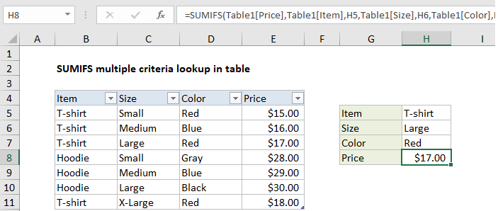
In some situations, you can use the SUMIFS function to perform multiple-criteria lookups on numeric data. To use SUMIFS like this, the lookup values must be numeric and unique to each set of possible criteria. In the example shown, the formula in H8 is:

=SUMIFS(Table1[Price],Table1[Item],H5,Table1[Size],H6,Table1[Color],H7)

Where Table1 is an Excel Table as seen in the screen shot.

How this formula works

This example shows how the SUMIFS function can sometimes be used to “lookup” numeric values, as an alternative to more complicated multi-criteria lookup formulas. This approach is less flexible than more general lookup formulas based on INDEX and MATCH (or VLOOKUP) but it’s also more straightforward, since SUMIFS is designed to easily handle multiple criteria. It’s also very fast.

In the example shown, we are using the SUMIFS function to “look up” the price of an item based on the item name, color, and size. The inputs for these criteria are the cells H5, H6, and H7.

Inside the SUMIFS function, the sum range is supplied as the “Price” column in Table1:

Table1[Price]

Criteria are supplied in 3 range/criteria pairs as follows:

Table1[Item],H5 // item
Table1[Size],H6 // size
Table1[Color],H7 // color

With this configuration, the SUMIFs function finds matching values in the “Price” column and returns the sum of matching prices for the specific criteria entered in H5:H7. Because only one price exists for each possible combination of criteria, the sum of the matching price is the same as as the sum of all matching prices.

Notes:

1. Each combination of criteria must match one result only.
2. Lookup values (the sum range) must be numeric.
3. SUMIFS will return zero if no match occurs.