Skip to content
xlsoffice. All Rights Reserved
  • Home
  • Excel For Beginners
  • Excel Intermediate
  • Advanced Excel For Experts

Lookup and Reference Examples

  • How to get address of last cell in range in Excel
  • How to use Excel COLUMN Function
  • How to get last row in numeric data in Excel
  • Offset in Excel
  • Find Closest Match in Excel Using INDEX, MATCH, ABS and MIN functions

Data Analysis Examples

  • How to Create Gantt Chart in Excel
  • Understanding Pivot Tables in Excel
  • How to perform a t-Test in Excel
  • Calculate Conditional Percentile ‘IF’ in table in Excel
  • How To Load Analysis ToolPak in Excel

Data Validation Examples

  • Excel Data validation must contain specific text
  • Excel Data validation don’t exceed total
  • Excel Data validation specific characters only
  • Data validation must not exist in list
  • Excel Data validation require unique number

Quickly Highlight Cells Containing Different Content in a Row

by

This example teaches you how to quickly highlight cells whose contents are different from the comparison cell in each row.

1. To select the range A1:C15, click on cell A1 and drag it to cell C15.

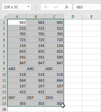
Note: because we selected the range A1:C15 by clicking on cell A1 first, cell A1 is the active cell (Use ENTER and TAB to change the active cell). As a result, the comparison cells are in column A.

Worked Example:   Convert Numbers to Text in Excel

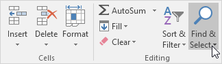
2. On the Home tab, in the Editing group, click Find & Select.

Worked Example:   How to create simple Time Sheet in Excel

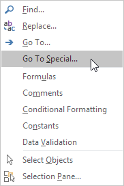
3. Click Go To Special.

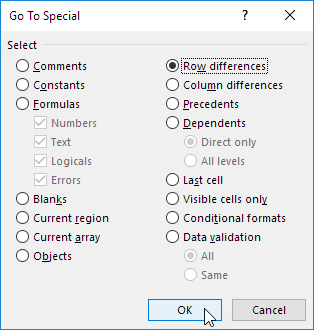
4. Select Row differences and click OK.

For row 2, Excel selects cell B2 because 523 is not equal to the value in cell A2 (522). For row 4, Excel selects cell B4 and cell C4 because 725 is not equal to the value in cell A4 (723), etc.

Worked Example:   Clean and reformat telephone numbers using SUBSTITUTE function in Excel

5. On the Home tab, in the Font group, change the background color of the selected cells.

Result:

Post navigation

Previous Post:

Conditional Formatting New Rule with Formulas in Excel

Next Post:

Delete Blank Rows at Once in Excel

Leave a Reply Cancel reply

Your email address will not be published. Required fields are marked *

Learn Basic Excel

Ribbon
Workbook
Worksheets
Format Cells
Find & Select
Sort & Filter
Templates
Print
Share
Protect
Keyboard Shortcuts

Categories

  • Charts
  • Data Analysis
  • Data Validation
  • Excel Functions
    • Cube Functions
    • Database Functions
    • Date and Time Functions
    • Engineering Functions
    • Financial Functions
    • Information Functions
    • Logical Functions
    • Lookup and Reference Functions
    • Math and Trig Functions
    • Statistical Functions
    • Text Functions
    • Web Functions
  • Excel VBA
  • Excel Video Tutorials
  • Formatting
  • Grouping
  • Others
  • Remove leading and trailing spaces from text in one or more cells in Excel
  • Put names into proper case — Manipulating NAMES in Excel
  • CONCAT function: Description, Usage, Syntax, Examples and Explanation
  • How to count specific characters in a cell in Excel
  • Split dimensions into two parts in Excel Worksheet
  • Display the current date in Excel
  • How to calculate quarter from date in Excel
  • Add decimal minutes to time in Excel
  • How to calculate nth day of year in Excel
  • YEARFRAC function: Description, Usage, Syntax, Examples and Explanation
  • INTRATE function: Description, Usage, Syntax, Examples and Explanation
  • RRI function: Description, Usage, Syntax, Examples and Explanation
  • COUPNUM function: Description, Usage, Syntax, Examples and Explanation
  • EFFECT function: Description, Usage, Syntax, Examples and Explanation
  • TBILLYIELD function: Description, Usage, Syntax, Examples and Explanation
Acronyms, Abbreviations, Initialism & What They Stand For
© 2022 xlsoffice . All Right Reserved. | Teal Smiles