Print Headers and Footers in Excel

This example teaches you how to add information to the header (top of each printed page) or footer (bottom of each printed page) in Excel.

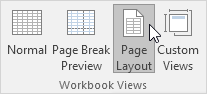
1. On the View tab, in the Workbook Views group, click Page Layout, to switch to Page Layout view.

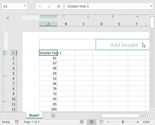
2. Click Add header.

The Header & Footer Tools contextual tab activates.

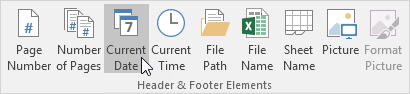
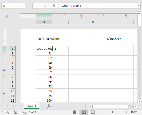
3. On the Design tab, in the Header & Footer Elements group, click Current Date to add the current date (or add the current time, file name, sheet name, etc).

Result:

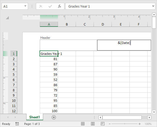
Note: Excel uses codes in order to automatically update the header or footer as you change the workbook.

4. You can also add information to the left and right part of the header. For example, click the left part to add the name of your company.

5. Click somewhere else on the sheet to see the header.

6. On the Design tab, in the Options group, you can add a different first page header/footer and a different header/footer for odd and even pages.

7. On the View tab, in the Workbook Views group, click Normal, to switch back to Normal view.