Get nth match in Excel

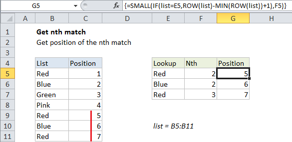
To get the position of the nth match (for example, the 2nd matching value, the 3rd matching value, etc.), you can use a formula based on the SMALL function. In the example shown, the formula in G5 is:

=SMALL(IF(list=E5,ROW(list)-MIN(ROW(list))+1),F5)

This formula returns the position of the second occurrence of “red” in the list.

Note: this is an array formula and must be entered with control + shift + enter.

How this formula works

This formula uses the named range “list” which is the range B5:B11.

The core of this formula is the SMALL function, which simply returns the nth smallest value in a list of values that correspond to row numbers. The row numbers have been “filtered” by the IF statement, which applies the logic for a match. Working from the inside out, IF compares all values in the named range “list” to the value in B5, which creates an array like this:

{TRUE;FALSE;FALSE;FALSE;TRUE;FALSE;TRUE}

The “value if true” is a set of relative row numbers created by this code:

ROW(list)-MIN(ROW(list))+1

The result is an array like this:

{1;2;3;4;5;6;7}

See this page for a full explanation.

With a logical test that returns an array of results, the IF function acts as a filter – only row numbers that correspond to a match survive, the rest return FALSE. The result returned by IF looks like this:

{1;FALSE;FALSE;FALSE;5;FALSE;7}

The numbers 1, 5, and 7 correspond to the location of “red” in the list.

Finally, SMALL returns the nth smallest item in this list, ignoring FALSE values. In the example, F5 contains 2, so SMALL returns the 2nd smallest value: 5.

Combine with INDEX

Once you have the relative position of the nth match, you can use that position inside of INDEX to return an associated value.