Count cells that contain negative numbers

This tutorial shows how to Count cells that contain negative numbers using the example below;

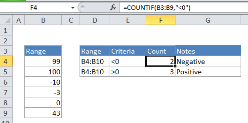
Formula

=COUNTIF(range,”<0″)

Explanation

To count the number of cells that contain negative numbers in a range of cells, you can use the COUNTIF function.

In the example, the active cell contains this formula:

=COUNTIF(B2:B6,"<0")

How this formula works

COUNTIF counts the number of cells in a range that match the supplied criteria. In this case, the criteria is supplied as “<0”, which is evaluated as “values less than zero”. The total count of all cells in the range that meet this criteria is returned by the function.

You can easily adjust this formula to count cells based on other criteria. For example, to count all cells with a value less -10, use this formula:

=COUNTIF(range,"<-10")

If you want to use a value in another cell as part of the criteria, use the ampersand (&) character to concatenate like this:

=COUNTIF(range,"<"&a1)

If the value in cell a1 is “-5”, the criteria will be “<-5” after concatenation.