Skip to content
Free Excel Tutorials
  • Home
  • Excel For Beginners
  • Excel Intermediate
  • Advanced Excel For Experts

Data Analysis

  • How To Sort One Column or Multiple Columns in Excel
  • Conflicting Multiple Conditional Formatting Rules in Excel
  • How To Insert and Customize Sparklines in Excel
  • Randomize/ Shuffle List in Excel
  • How To Create Pareto Chart in Excel

References

  • How to get last row in numeric data in Excel
  • How to retrieve first match between two ranges in Excel
  • How to use Excel TRANSPOSE Function
  • Approximate match with multiple criteria in Excel
  • Extract data with helper column in Excel

Data Validations

  • Excel Data validation whole percentage only
  • Excel Data validation exists in list
  • Excel Data validation don’t exceed total
  • Excel Data validation must begin with
  • Excel Data validation date in specific year

3D sum multiple worksheets in Excel

by

This tutorial shows how to 3D sum multiple worksheets in Excel using the example below;

Formula

=SUM(Sheet1:Sheet3!A1)

Explanation

To sum the same range in one or more sheets, you can use the SUM formula with a special syntax called a “3d reference”.

Worked Example:   Average last 5 values in columns in Excel

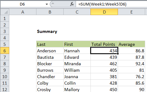
In the example shown, the formula in D6 is:

=SUM(Week1:Week5!D6)

How this formula works

The syntax for referencing a range of sheets is a built-in feature and works a bit like a reference to a range of cells. For example

Sheet1:Sheet3!A1

Means: cell A1 from Sheet1 to Sheet3.

Worked Example:   Average last 5 values in Excel

In the example shown:

=SUM(Week1:Week5!D6)

Will sum cell D6 from Week1 to Week5, equivalent to:

=SUM(Week1!D6,Week2!D6,Week3!D6,Week4!D6,Week5!D6)

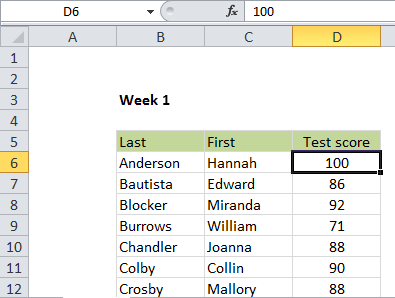
In this workbook, the sheets Week1 through Week 6 all look exactly like this:

Worked Example:   How to calculate average last N values in a table in Excel

Other examples

You can use 3D references in other formulas as well. For example, the formula in E6 averages D6 like this:

=AVERAGE(Week1:Week5!D6)

Post navigation

Previous Post:

How to use Excel FALSE Function

Next Post:

Large with criteria in Excel

Leave a Reply Cancel reply

Your email address will not be published. Required fields are marked *

Learn Basic Excel

Ribbon
Workbook
Worksheets
Format Cells
Find & Select
Sort & Filter
Templates
Print
Share
Protect
Keyboard Shortcuts

Categories

  • Charts
  • Data Analysis
  • Data Validation
  • Excel Functions
    • Cube Functions
    • Database Functions
    • Date and Time Functions
    • Engineering Functions
    • Financial Functions
    • Information Functions
    • Logical Functions
    • Lookup and Reference Functions
    • Math and Trig Functions
    • Statistical Functions
    • Text Functions
    • Web Functions
  • Excel VBA
  • Excel Video Tutorials
  • Formatting
  • Grouping
  • Others

Logical Functions

  • How to use Excel OR Function
  • IF function: Description, Usage, Syntax, Examples and Explanation
  • How to return blank in place of #DIV/0! error in Excel
  • Nested IF function example in Excel
  • Invoice status with nested if in Excel

Date Time

  • List holidays between two dates in Excel
  • Get project midpoint in Excel
  • NETWORKDAYS function: Description, Usage, Syntax, Examples and Explanation
  • How to calculate Next working/business day in Excel
  • Add decimal minutes to time in Excel

Grouping

  • Map text to numbers in Excel
  • How to randomly assign data to groups in Excel
  • Group numbers at uneven intervals in Excel
  • How to randomly assign people to groups in Excel
  • Calculate conditional mode with criteria in Excel

General

  • How to choose page/paper size in Excel before Printing
  • How to get Excel workbook path only
  • Find Most Frequently Occurring Word in Excel Worksheet
  • Convert column letter to number in Excel
  • How to count total columns in range in Excel
© 2023 xlsoffice . All Right Reserved. | Teal Smiles | Abbreviations And Their Meaning