Highlight data by quartile in Excel

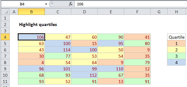
This tutorial shows how to Highlight data by quartile in Excel using the example below;

Formula

=A1>=QUARTILE(data,quart)

Explanation

To highlight cells by quartile, you can apply conditional formatting with a formula that uses the QUARTILE function.

In the example shown, we are using 4 different conditional formatting rules. Each rule highlights a quartile in the range B4:F11 using the QUARTILE function. The formulas look like this:

=B4>QUARTILE(B4:F11,3)
=B4>=QUARTILE(B4:F11,2)
=B4>=QUARTILE(B4:F11,1)
=B4>=QUARTILE(B4:F11,0)

Note that we are highlighting quartiles in a specific order, starting with quartile 4 and ending with quartile 1.

It’s important that the formula be entered relative to the upper left most cell in the data, in this case cell B4.

How this formula works

The QUARTILE function is automatic, and will calculate the 1st quartile with an input of 1, the 2nd quartile with an input of 2, and the 3rd quartile with an input of 3. With an input of 0, quartile returns the minimum value in the data.

The trick in this case is to arrange the conditional formatting rules so that they run in the same direction. The first rule highlights values greater than the 3rd quartile. The second rule highlights values greater than the 2nd quartile, the 3rd rule highlights data greater than the 1st quartile, and the last rule highlights data greater than the minimum value.