Highlight approximate match lookup conditional formatting in Excel

This tutorial shows how to Highlight approximate match lookup conditional formatting in Excel using the example below;

Formula

=OR($B5=LOOKUP(width,widths),B$5=LOOKUP(height,heights))

Explanation

To highlight rows and columns associated with an approximate match, you can use conditional formatting with a formula based on the LOOKUP function together with with a logical function like OR or AND. In the example shown, the formula used to apply conditional formatting is:

=OR($B5=LOOKUP(width,widths),B$5=LOOKUP(height,heights))

How this formula works

This formula uses 4 named ranges, defined as follows:

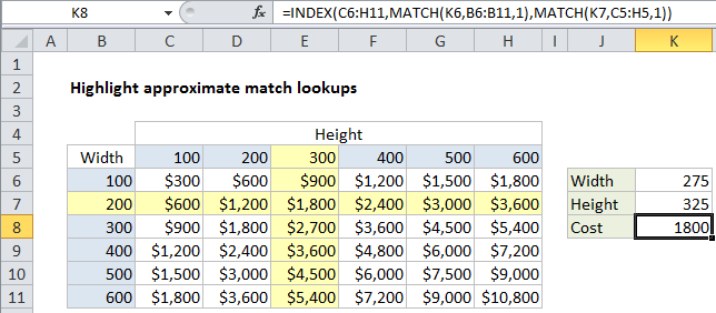
width=K6
height=K7
widths=B6:B11
heights=C5:H5

Conditional formatting is evaluated relative to every cell it is applied to, starting with the active cell in the selection, which is cell B5 in this case. To highlight the matching row, we use this logical expression:

$B5=LOOKUP(width,widths)

The reference to B5 is mixed, with the column locked and row unlocked, so that only values in column B (widths) are compared to the value in K6 (width). In the example shown, this logical expression will return TRUE for every cell in a row where width is 200, based on an approximate match of the value in K6 (width, 275) against all values in K6:B11 (widths). This is done with LOOKUP function:

LOOKUP(width,widths)

Like the MATCH function, LOOKUP will run through sorted values until a greater value is found, then “step back” to the previous value, which is 200 in this case.

To highlight the matching column, we use this logical expression:

B$5=LOOKUP(height,heights)

The reference to B5 is mixed, with the column relative and row absolute, so that only values in row 5 (heights) are compared to the value in K7 (height). In the example shown, this logical expression will return TRUE for every cell in a row where height is 300, based on an approximate match of the value in K7 (height, 325) against all values in C5:H5 (heights). This is done with LOOKUP function:

LOOKUP(height,heights)

As above, LOOKUP will run through sorted values until a greater value is found, then “step back” to the previous value, which is 300 in this case.

Highlight intersection only

To highlight the intersection only, just replace the OR function with the AND function:

=AND($B5=LOOKUP(width,widths),B$5=LOOKUP(height,heights))