How to strip numeric characters from cell in Excel

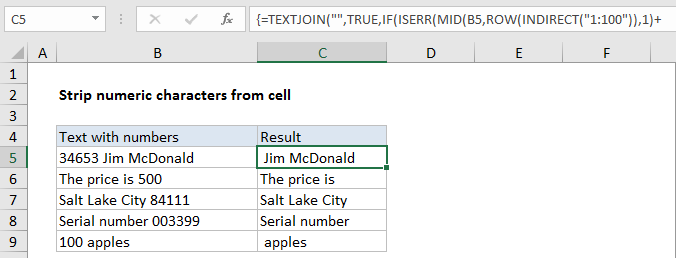
In the example shown, the formula in C5 is:

=TEXTJOIN("",TRUE,IF(ISERR(MID(B5,
ROW(INDIRECT("1:100")),1)+0),
MID(B5,ROW(INDIRECT("1:100")),1),""))

Note: this is an array formula and must be entered with control + shift + enter.

How this formula works

Working from the inside out, the MID formula is used to extract the text in B5, one character at a time.  The key is the ROW/INDIRECT piece:

ROW(INDIRECT("1:100"))

which spins up an array containing 100 numbers like this:

{1,2,3,4,5,6,7,8….99,100}

Note: 100 represents the maximum characters to process. Change to suit your data.

This array goes into the MID function as the start_num argument. For num_chars, we use 1.

The MID function returns an array like this:

{“3″;”4″;”6″;”5″;”3″;” “;”J”;”i”;”m”;” “;”M”;

“c”;”D”;”o”;”n”;”a”;”l”;”d”;””;””;””;…}

(extra items in the array removed for readability)

To this array, we add zero. This is a simple trick that forces Excel to try and coerce text to a number. Numeric text values like “1”,”2″,”3″,”4″ etc. are converted, while non-numeric values fail and throw a #VALUE error. We use the IF and ISERR functions to catch these errors. If get an error we know we have a non-numeric character, so we use another MIN function to bring it into our array:

MID(B5,ROW(INDIRECT("1:100")),1)

If don’t get an error, we know we have a number, so we just insert an empty string (“”) into the array.

The final array result goes into the TEXTJOIN function as the text1 argument. For delimiter, we use an empty string (“”) and for ignore_empty we supply TRUE. TEXTJOIN then concatenates all non-empty values in the array and returns the result.

More precise array length

If it bothers you to hard-code a value like 100 into INDIRECT, you can use the LEN function inside INDIRECT to more intelligently process only the actually number of characters in the cell.

MID(A1,ROW(INDIRECT("1:"&LEN(A1))),1)

Removing extra space

When you strip numeric characters, you may have extra space characters left over. To strip leading and trailing spaces, and normalize spaces between words, you can wrap the formula shown on this page inside the TRIM function:

=TRIM(formula)