Skip to content
Free Excel Tutorials
  • Home
  • Excel For Beginners
  • Excel Intermediate
  • Advanced Excel For Experts

Data Analysis

  • Excel Pie Chart
  • Conditional Formatting New Rule with Formulas in Excel
  • Remove Duplicates Example in Excel
  • How to create running total in an Excel Table
  • Example of COUNTIFS with variable table column in Excel

References

  • How to get last row in mixed data with blanks in Excel
  • Excel Advanced Lookup using Index and Match Functions
  • Extract all partial matches in Excel
  • Complete List of Excel Lookup and Reference Functions, References and Examples
  • How to use Excel INDIRECT Function

Data Validations

  • Excel Data validation don’t exceed total
  • Excel Data validation number multiple 100
  • Excel Data validation date in specific year
  • How To Create Drop-down List in Excel
  • Data validation must not exist in list

How to extract last two words from text string in Excel

by

To extract the last two words from a cell, you can use a formula built with several Excel functions, including MID, FIND, SUBSTITUTE, and LEN.

Formula

=MID(A1,FIND("@",SUBSTITUTE(A1," ","@",LEN(A1)-LEN(SUBSTITUTE(A1," ",""))-1))+1,100)

Explanation

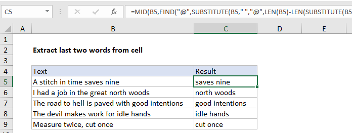
In the example shown, the formula in C5 is:

=MID(B5,FIND("@",SUBSTITUTE(B5," ","@",LEN(B5)-LEN(SUBSTITUTE(B5," ",""))-1))+1,100)

How this formula works

At the core, this formula uses the MID function to extract characters starting at the second to last space.  The MID function takes 3 arguments: the text to work with, the starting position, and the number of characters to extract.

The text comes from column B, and the number of characters can be any large number that will ensure the last two words are extracted. The challenge is to determine the starting position, which is just after the second to last space. The clever work is done primarily with the SUBSTITUTE function, which has an optional argument called instance number.  This feature is used to replace the second to last space in the text with the “@” character, which is then located with the FIND function.

Working from the inside out, the snippet below figures out how many spaces are in the text total, from which 1 is subtracted.

LEN(B5)-LEN(SUBSTITUTE(B5," ",""))-1

In the example shown, there are 5 spaces in the text, so the code above returns 4. This number is fed into the outer SUBSTITUTE function as instance number:

SUBSTITUTE(B5," ","@",4)

This causes SUBSTITUTE to replace the forth space character with “@”. The choice of @ is arbitrary. You can use any character that will not appear in the original text.

Next, the FIND locates the “@” character in the text:

FIND("@","A stitch in time@saves nine")

The result of FIND is 17, to which 1 is added to get 18. This is the starting position, and goes into the MID function as the second argument. For simplicity, the number of characters to extract is hardcoded as 100. This number is arbitrary and can be adjusted to fit the situation.

Extract last N words from cell

This formula can be generalized to extract the last N words from a cell by replacing the hardcoded 1 in the example with (N-1). In addition, if you are extracting many words, you may want to replace the hardcoded argument in MID, 100, with a larger number. To guarantee you the number is large enough, you could simply use the LEN function as follows:

=MID(B5,FIND("@",SUBSTITUTE(B5," ","@",LEN(B5)-LEN(SUBSTITUTE(B5," ",""))-(N-1)))+1,LEN(B5))

Post navigation

Next Post:

Create One-dimensional and Two-dimensional Array

Leave a Reply Cancel reply

Your email address will not be published. Required fields are marked *

Learn Basic Excel

Ribbon
Workbook
Worksheets
Format Cells
Find & Select
Sort & Filter
Templates
Print
Share
Protect
Keyboard Shortcuts

Categories

  • Charts
  • Data Analysis
  • Data Validation
  • Excel Functions
    • Cube Functions
    • Database Functions
    • Date and Time Functions
    • Engineering Functions
    • Financial Functions
    • Information Functions
    • Logical Functions
    • Lookup and Reference Functions
    • Math and Trig Functions
    • Statistical Functions
    • Text Functions
    • Web Functions
  • Excel VBA
  • Excel Video Tutorials
  • Formatting
  • Grouping
  • Others

Logical Functions

  • How to return blank in place of #DIV/0! error in Excel
  • How to use Excel NOT Function
  • XOR function: Description, Usage, Syntax, Examples and Explanation
  • IF with wildcards in Excel
  • IFS function: Description, Usage, Syntax, Examples and Explanation

Date Time

  • Add workdays to date custom weekends in Excel
  • WEEKNUM function: Description, Usage, Syntax, Examples and Explanation
  • Next biweekly payday from date in Excel
  • Calculate expiration date in Excel
  • TODAY function: Description, Usage, Syntax, Examples and Explanation

Grouping

  • How to randomly assign data to groups in Excel
  • Categorize text with keywords in Excel
  • If cell contains one of many things in Excel
  • Group arbitrary text values in Excel
  • Calculate conditional mode with criteria in Excel

General

  • Sum by group in Excel
  • Creating and Opening an existing file in Excel
  • How to get amount with percentage in Excel
  • Select, Insert, Rename, Move, Delete Worksheets in Excel
  • Convert column number to letter in Excel
© 2026 xlsoffice . All Right Reserved. | Teal Smiles | Abbreviations And Their Meaning