Extract date from a date and time in Excel

This tutorial show how to Extract date from a date and time in Excel using the example below.

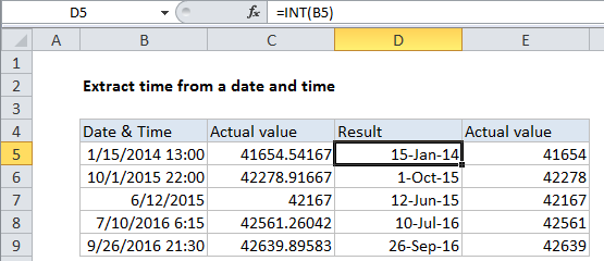
If you have dates with time values and you want to extract only the date portion, you can use a formula that uses the INT function.

Note: Excel handles dates and time using a scheme in which dates are serial numbers and times are fractional values. For example, June 1, 2000 12:00 PM is represented in Excel as the number 36678.5, where 36678 is the date portion and .5 is the time portion.

Formula

=INT(date)

Explanation of how this formula works

So, assuming A1 contains the date and time, June 1, 2000 12:00 PM, the formula below returns just the date portion (36678):

=INT(A1)

The time portion of the value (the fractional part) is discarded. You could also use the TRUNC function with the same result:

=TRUNC(A1)

Notes:

1. With either method above, make sure you use a date format on the result that does not include a time. Otherwise, you’ll see the time displayed as 12:00 AM.

2. For dates and times (which must be positive in Excel) there is no difference in using INT and TRUNC to extract an integer. But INT actually rounds numbers down to the nearest integer, which makes a difference when values are negative.