Count missing values in Excel

To count the values in one list that are missing from another list, you can use a formula based on the COUNTIF and SUMPRODUCT functions.

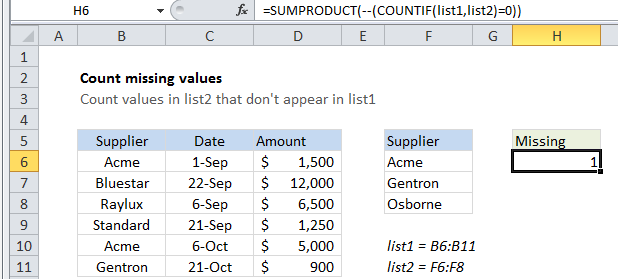
In the example shown, the formula in H6 is:

=SUMPRODUCT(--(COUNTIF(list1,list2)=0))

Which returns 1 since the value “Osborne” does not appear in B6:B11.

How this formula works

The COUNTIF functions checks values in a range against criteria. Often, only one criteria is supplied, but in this case we supply more than one criteria.

For range, we give COUNTIF the named range list1 (B6:B11), and for criteria, we provide the named range list2 (F6:F8).

Because we give COUNTIF more than one criteria, we get more than one result in a result array that looks like this: {2;1;0}

We want to count only values that are missing, which by definition have a count of zero, so we convert these values to TRUE and FALSE with the “=0” statement, which yields: {FALSE;FALSE;TRUE}

Then we force the TRUE FALSE values to 1s and 0s with the double-negative operator (–), which produces: {0;0;1}

Finally, we use SUMPRODUCT to add up the items in the array and return a total count of missing values.

Alternative with MATCH

If you prefer more literal formulas, you can use the formula below, based on MATCH, which literally counts values that are “missing” using the ISNA function:

=SUMPRODUCT(--ISNA(MATCH(list2,list1,0)))