Basic Tax Rate calculation with VLOOKUP in Excel

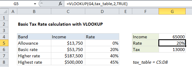
To calculate a tax rate based on a simple tax rate table, you can use the VLOOKUP function. In the example shown, the formula in G5 is:

=VLOOKUP(G4,tax_table,2,TRUE)

How this formula works

Note: This formula depends on a simple tax table with numeric data in the first column, sorted from lowest to highest. The first column in the table represents “lookup values”.

The solution requires only the VLOOKUP function:

• The lookup value itself comes from G4
• The table array is the named range tax_table
• The column index number is 2, since the actual tax rates are in the second column
• Finally, the range_lookup argument is set to TRUE, to allow an approximate match

With this configuration, VLOOKUP scans the lookup values until it finds a value higher than the value in G4, then VLOOKUP “drops back” to the previous row and returns the tax rate from the second column in the table.

VLOOKUP matching modes

VLOOKUP has two matching modes: exact match and approximate match, controlled by the forth argument, called range_lookup. The range_lookup argument is optional and defaults to TRUE, but in this case it is set explicitly to TRUE for clarity.