Minimum if multiple criteria in Excel

Formula

{=MIN(IF(range1=criteria1,IF(range2=criteria2,values)))}

Explanation

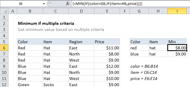
In the example shown the formula in I6 is:

{=MIN(IF(color=G6,IF(item=H6,price)))}

With a color of “red” and item of “hat” the result is $8.00

Note: This is an array formula and must be entered using Ctrl + Shift + entered

How this formula works

This example uses the following named ranges: “color” = B6:B14, “item” = C6:C14, and “price” = E6:E14. In the example, we have pricing on items in various regions. The goal is to find the minimum price for a given color and item.

This formula uses two nested IF functions, wrapped inside MIN to return the minimum price using two criteria. Starting with logical test of the first IF statement, color = G6, the values in the named range color (B6:B14) are checked against the value in cell G6, “red”. The result is an array like this:

{TRUE;TRUE;TRUE;FALSE;FALSE;FALSE;FALSE;FALSE;FALSE}

In the logical test for the second IF statement, item = H6, the values in the named range item (C6:C14) are checked against the value in cell H6, “hat”. The result is an array like this:

{TRUE;TRUE;TRUE;TRUE;TRUE;TRUE;FALSE;FALSE;FALSE}

The “value if true” for the 2nd IF statement the named range “prices” (E6:E14), which is an array like this:

{11;8;9;12;9;10;9;8;7}

A price is returned for each item in this range only when the result of the first two arrays above is TRUE for items in corresponding positions. In the example shown the final array inside of MIN looks like this:

{11;8;9;FALSE;FALSE;FALSE;FALSE;FALSE;FALSE}

Note the only prices that “survive” are those in a position where the color is “red” and the item is “hat”.

The MIN function then returns the lowest price, automatically ignoring FALSE values.

Alternative syntax using boolean logic

You can also use the following array formula, which uses only one IF function together with boolean logic:

{=MIN(IF((color=G6)*(item=H6),price))}

The advantage of this syntax is that it is arguably easier to add additional criteria without adding additional nested IF functions.

With MINIFS function

The MINIFS function, introduced in Excel 2016 via Office 365, is designed to return minimums based on one or more criteria, without the need for an array formula. With MINIFS, the formula in I6 becomes:

=MINIFS(price,color,G6,item,H6)