Sumproduct Function Example in Excel

To calculate the sum of the products of corresponding numbers in one or more ranges, use Excel’s powerful SUMPRODUCT function.

Basic Use

1. For example, the SUMPRODUCT function below calculates the total amount spent.

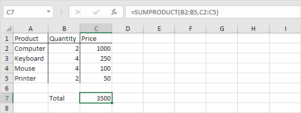
Explanation: the SUMPRODUCT function performs this calculation: (2 * 1000) + (4 * 250) + (4 * 100) + (2 * 50) = 3500.

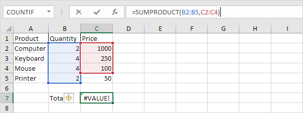
2. The ranges must have the same dimensions or Excel will display the #VALUE! error.

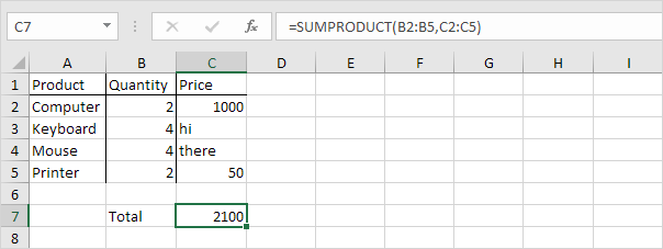
3. The SUMPRODUCT function treats any entries that are not numeric as if they were zeros.

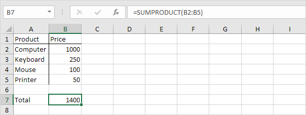
4. If you supply a single range, the SUMPRODUCT function produces the exact same result as the SUM function.

Advanced Use

The SUMPRODUCT function is an extremely versatile function and can produce the same result as many built-in functions in Excel and even array formulas!

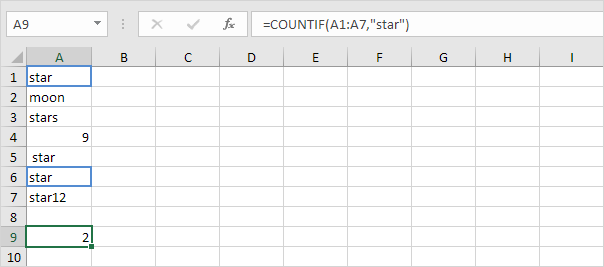
1a. For example, the COUNTIF function below counts the number of cells that contain exactly star.

1b. The SUMPRODUCT function below produces the exact same result.

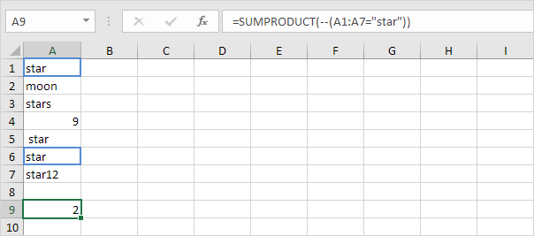
Explanation: –(A1:A7=”star”) reduces to the following array constant:

–{TRUE;FALSE;FALSE;FALSE;FALSE;TRUE;FALSE}

The double negative — coerces these Booleans to 1’s and 0’s (TRUE=1, FALSE=0). Result:

{1;0;0;0;0;1;0}

This array constant is used as an argument for the SUMPRODUCT function, giving a result of 2.

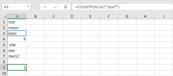
1c. The COUNTIF function below counts the number of cells that contain exactly star + 1 character. A question mark (?) matches exactly one character.

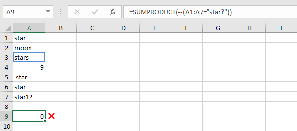
1d. The SUMPRODUCT function is not perfect! You cannot use wildcard characters (? and *) when you use the SUMPRODUCT function.

2a. The array formula below counts the number of characters in a range of cells.

Note: finish an array formula by pressing CTRL + SHIFT + ENTER. Excel adds the curly braces {}.

2b. The SUMPRODUCT function below produces the exact same result.

Note: the array constant {9;4;6;5} is used as an argument for the SUMPRODUCT function, giving a result of 24. The SUMPRODUCT function handles arrays natively so you don’t have to finish by pressing CTRL + SHIFT + ENTER. This is one of the biggest advantages of the SUMPRODUCT function because the curly braces {} confuse many Excel beginners!

3a. The array formula below sums the sales in 2018.

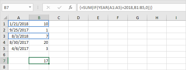
3b. The SUMPRODUCT function below produces the exact same result.

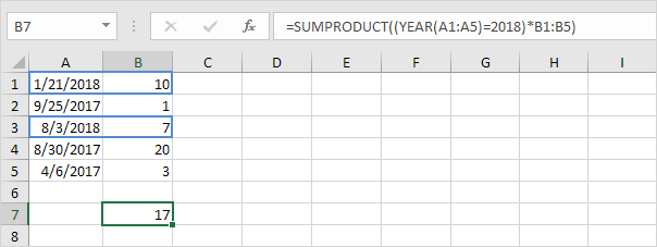
Explanation: (YEAR(A1:A5)=2018)*B1:B5 reduces to:

({2018;2017;2018;2017;2017}=2018)*{10;1;7;20;3} and this reduces to:

{TRUE;FALSE;TRUE;FALSE;FALSE}*{10;1;7;20;3}

We don’t need a double negative (see example 1b) because the multiplication operator * automatically coerces the Booleans to 1’s and 0’s (TRUE=1, FALSE=0). Result:

{10;0;7;0;0}

This array constant is used as an argument for the SUMPRODUCT function, giving a result of 17.