SUMIFS with multiple criteria and OR logic in Excel

=SUM(SUMIFS(sum_range,criteria_range,{"red","blue"}))

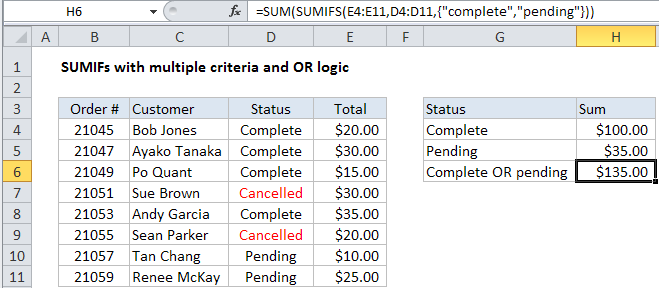
To sum based on multiple criteria using OR logic, you can use the SUMIFS function with an array constant. In the example shown, the formula in H6 is:

=SUM(SUMIFS(E4:E11,D4:D11,{"complete","pending"}))

How this formula works

By default, the SUMIFS function only allows AND logic – when you provide multiple conditions, all conditions must match to be included in the result.

One solution is to supply multiple criteria in an array constant like this:

{“complete”,”pending”}

This will cause SUMIFS to return two results: a count for “complete” and a count for “pending”, in an array result like this:

{100,35}

To get a final total, we wrap SUMIFS inside SUM. The SUM function sums all items in the array and returns the result.

Cell references for criteria

You can’t use cell references inside an array constant. To use a cell reference for criteria, you can use an array formula like this:

={SUM(SUMIFS(range1,range2,range2))}

Where range1 is the sum range, range2 is the criteria range, and range3 contains criteria on the worksheet. With two OR criteria, you’ll need to use horizontal and vertical arrays.

Note: this is an array formula and must be entered with control + shift + enter.

With wildcards

You can use wildcards in the criteria if needed. For example, to sum items that contain “red” or “blue” anywhere in the the criteria_range, you can use:

=SUM(SUMIFS(sum_range,criteria_range,{"*red*","*blue*"}))

Adding another OR criteria

You can add one additional criteria to this formula, but you’ll need to use a single column arrayfor one criteria and a single row array for the other. So, for example, to sum orders that are “Complete” or “Pending”, for either “Andy Garcia” or “Bob Jones”, you can use:

=SUM(SUMIFS(E4:E11,D4:D11,{"complete","pending"},C4:C11,{"Bob Jones";"Andy Garcia"}))

Note the semi-colons in the second array constant, which represents a vertical array. This works because Excel “pairs” elements in the two array constants, and returns a two dimensional array of results. With more criteria, you will want to move to a formula based on SUMPRODUCT.