Sum top n values with criteria in Excel

=SUMPRODUCT(LARGE((range=criteria)*(values),{1,2,3,N}))

To sum the top n values in a range matching criteria, you can use a formula based on the LARGE function, wrapped inside the SUMPRODUCT function. In the generic form of the formula (above), range represents a range of cells that are compared to criteria, values represents numeric values from which top values are retrieved, and N represents the idea of Nth value.

In the example, the active cell contains this formula:

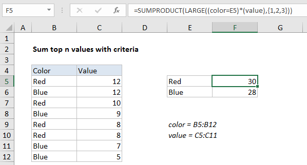
=SUMPRODUCT(LARGE((color=E5)*(value),{1,2,3}))

Where color is the named range B5:B12 and value is the named range C5:C12.

Here’s how the formula works

In its simplest form, LARGE returns the “Nth largest” value in a range with this construction:

=LARGE (range,N)

So, for example:

=LARGE (C5:C12,2)

will return the 2nd largest value in the range C5:C12, which is 12 in the example shown.

However, if you supply an “array constant” (e.g. a constant in the form {1,2,3}) to LARGE as the second argument, LARGE will return an array of results instead of a single result. So, the formula:

=LARGE (C5:C12, {1,2,3})

will return the 1st, 2nd, and 3rd largest value C5:C12 in an array like this:{12,12,10}

So, the trick here is to filter the values based on color before LARGE runs. We do this with the expression:

(color=E5)

Which results in an array of TRUE / FALSE values. During the multiplication operation, these values are coerced into ones and zeros:

=LARGE({1;0;1;0;1;1;0;0}*{12;12;10;9;8;8;7;5},{1,2,3})

So the final result is that only values associated with the color “red” survive the operation:

=SUMPRODUCT(LARGE({12;0;10;0;8;8;0;0},{1,2,3}))

and the other values are forced to zero.

Note: this formula won’t handle text in the value range. See below.

Handling text in values

If you have text anywhere in the value ranges, the LARGE function will throw a #VALUE error and stop the formula from working.

To handle text in the value range, you can add the IFERROR function like this:

=SUM(IFERROR(LARGE(IF((color=E5),value),{1,2,3}),0))

Here, we trap errors from LARGE caused by text values and replace with zero. Using IF inside LARGE requires that the formula be entered with control + shift + enter, so we switch to SUM instead of SUMPRODUCT.