Sum if cell contains text in another cell in Excel

This tutorial shows how to Sum if cell contains text in another cell in Excel using the example below;

Formula

=SUMIF(range,"*"&A1&"*",sum_range)

Explanation

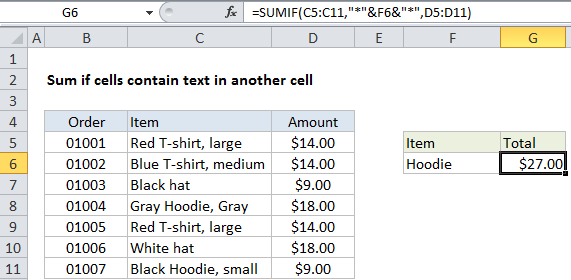
To sum if cells contain specific text in another cell, you can use the SUMIF function with a wildcard and concatenation. In the example shown, cell G6 contains this formula:

=SUMIF(C5:C11,"*"&F6&"*",D5:D11)

This formula sums amounts for items in column C that contain “hoodie”, anywhere in the cell.

How the formula works

The SUMIF function supports wildcards. An asterisk (*) means “zero or more characters”, while a question mark (?) means “any one character”.

Wildcards allow you to create criteria such as “begins with”, “ends with”, “contains 3 characters” and so on.

So, for example, you can use “*hat*” to match the text “hat” anywhere in a cell, or “a*” to match values beginning with the letter “a”.

In this case, we want to match the text in F6. We can’t write the criteria like “*F6*” because that will match only the literal text “F6”.

Instead, we need to use the concatenation operator (&) to join a reference to F6 to asterisks (*):

"*"&F6&"*"

When Excel evaluates this argument inside the SUMIF function, it will “see” “*hoodie*” as the criteria:

=SUMIF(C5:C11,"*hoodie*",D5:D11)

SUMIF then returns the sum for items that contain “hoodie”, which is $27.00 in the example shown.

Note that SUMIF is not case-sensitive.

Alternative with SUMIFS

You can also use the SUMIFS function. SUMIFS can handle multiple criteria, and the order of the arguments is different from SUMIF. The equivalent SUMIFS formula is:

=SUMIFS(D5:D11,C5:C11,"*"&F6&"*")

Notice the sum range always comes first in the SUMIFS function.