
Skip to content
Free Excel Tutorials
  • Home
  • Excel For Beginners
  • Excel Intermediate
  • Advanced Excel For Experts

Data Analysis

  • How to Create Column Chart in Excel
  • How to calculate current stock or inventory in Excel
  • How to Create Thermometer Chart in Excel
  • Randomize/ Shuffle List in Excel
  • What-If Analysis: Scenarios and Goal Seek in Excel

References

  • Last row number in range
  • Get nth match with INDEX / MATCH in Excel
  • How to get relative row numbers in a range in Excel
  • Create hyperlink with VLOOKUP in Excel
  • Left Lookup in Excel

Data Validations

  • Data validation must not exist in list
  • How To Create Drop-down List in Excel
  • Excel Data validation number multiple 100
  • Prevent invalid data entering in specific cells
  • Excel Data validation allow uppercase only

Sum entire column in Excel

by

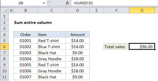
This tutorial shows how to Sum entire column in Excel using the example below;

Formula

=SUM(A:A)
Explanation

If you want to sum an entire column without supplying an upper or lower bound, you can use the SUM function with and the specific range syntax for entire column.

In the example shown, the formula in G6 is:

=SUM(D:D)

How this formula works

Excel supports “full column” and “full row” references like this:

=SUM(A:A) // sum all of column A
=SUM(3:3) // sum all of row 3

You can see how this works yourself by typing “A:A”, “3:3”, etc. into the name box (left of the formula bar) and hitting return — Excel will select the entire column or row.

Note: Full column and row references are an easy way to reference data that may change in size, but you need to be sure that you aren’t unintentionally including extra data. For example, if you use =SUM(A:A:) to sum all of column A, and column A also includes a date somewhere (anywhere), this date will be included in the sum.

Post navigation

Previous Post:

How to use Excel CHOOSE Function

Next Post:

Customize Ribbon In Excel

Leave a Reply Cancel reply

Your email address will not be published. Required fields are marked *

Learn Basic Excel

Ribbon
Workbook
Worksheets
Format Cells
Find & Select
Sort & Filter
Templates
Print
Share
Protect
Keyboard Shortcuts

Categories

  • Charts
  • Data Analysis
  • Data Validation
  • Excel Functions
    • Cube Functions
    • Database Functions
    • Date and Time Functions
    • Engineering Functions
    • Financial Functions
    • Information Functions
    • Logical Functions
    • Lookup and Reference Functions
    • Math and Trig Functions
    • Statistical Functions
    • Text Functions
    • Web Functions
  • Excel VBA
  • Excel Video Tutorials
  • Formatting
  • Grouping
  • Others

Logical Functions

  • Complete List of Excel Logical Functions, References and Examples
  • How to use Excel XOR Function
  • IFERROR function: Description, Usage, Syntax, Examples and Explanation
  • IF with boolean logic in Excel
  • How to return blank in place of #DIV/0! error in Excel

Date Time

  • Get last working day in month in Excel
  • How to calculate most recent day of week in Excel
  • WEEKNUM function: Description, Usage, Syntax, Examples and Explanation
  • SECOND function: Description, Usage, Syntax, Examples and Explanation
  • YEAR function: Description, Usage, Syntax, Examples and Explanation

Grouping

  • Group arbitrary text values in Excel
  • Calculate conditional mode with criteria in Excel
  • Group numbers with VLOOKUP in Excel
  • Map text to numbers in Excel
  • Map inputs to arbitrary values in Excel

General

  • Share Excel data with Word documents
  • How to create dynamic named range with INDEX in Excel
  • Mark Workbook as Final in Excel
  • How to count total number of cells in a rectangular range in Excel
  • How to choose page/paper size in Excel before Printing
© 2026 xlsoffice . All Right Reserved. | Teal Smiles | Abbreviations And Their Meaning