Sum 2d range with multiple criteria in Excel

This tutorial shows how to Sum 2d range with multiple criteria in Excel using the example below;

To lookup and sum values in a 2D range with multiple criteria, you can use the SUMPRODUCT function.

Formula

=SUMPRODUCT(data*(range1=criteria1)*(range2=criteria2))

Explanation

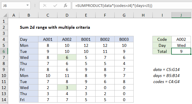
In the example shown, the formula in J6 is:

=SUMPRODUCT(data*(codes=J4)*(days=J5))

using named ranges as shown in the image.

How this formula works

The SUMPRODUCT function can handle arrays natively, without requiring control shift enter.

In this case, we are multiplying all values in the named range data by two expressions that filter out values not of interest. The first expression applies a filter based on codes:

(codes=J4)

Since J4 contains “A002”, the expression creates an array of TRUE FALSE values like this:

{FALSE,TRUE,FALSE,FALSE,FALSE}

The second expression filters on day:

(days=J5)

Since J4 contains “Wed”, the expression creates an array of TRUE FALSE values like this:

{FALSE;FALSE;TRUE;FALSE;FALSE;FALSE;FALSE;TRUE;FALSE;FALSE}

In Excel TRUE FALSE values are automatically coerced to 1 and 0 values by any math operation, so the multiplication operation coerces the arrays above to ones and zeros, and creates a 2D array with the same dimensions as the original data. The process can be visualized as shown below:

Finally, SUMPRODUCT returns the sum of all elements in the final array, 9.