How to use Excel HLOOKUP Function

This Excel tutorial explains how to use the HLOOKUP function with syntax and examples. How to handle errors such as #N/A and retrieve the correct results is also discussed.

Excel HLOOKUP function Description

The Microsoft Excel HLOOKUP function performs a horizontal lookup by searching for a value in the top row of the table and returning the value in the same column based on the index_number.

The HLOOKUP function is a built-in function in Excel that is categorized as a Lookup/Reference Function. HLOOKUP function can be entered as part of a formula in a cell of a worksheet.

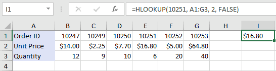
Explanation: The above HLOOKUP examples would return:

=HLOOKUP(10251, A1:G3, 2, FALSE)
Result: $16.80    'Returns value in 2nd row

=HLOOKUP(10251, A1:G3, 3, FALSE)
Result: 6         'Returns value in 3rd row

=HLOOKUP(10248, A1:G3, 2, FALSE)
Result: #N/A      'Returns #N/A error (no exact match)

=HLOOKUP(10248, A1:G3, 2, TRUE)
Result: $14.00    'Returns an approximate match