First match in range with wildcard in Excel

This tutorial shows how to calculate First match in range with wildcard in Excel using the example below;

Formula

=INDEX(range,MATCH(val&"*",range,0))

Explanation

To get the value of the first match in a range using a wildcard, you can use an INDEX and MATCH formula, configured for exact match.

In the example shown, the formula in F5 is:

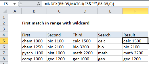
=INDEX(B5:D5,MATCH(E5&"*",B5:D5,0))

How this formula works

Working from the inside out, MATCH is used to locate the position of the first match in the range B5:D5. The lookup_value is based on the value in B5 joined with an asterisk (*) as a wildcard, and match_type is set to zero to force an exact match:

MATCH(E5&"*",B5:D5,0)

E5 contains the string “calc” so, after concatenation, the MATCH function looks like this:

MATCH("calc*",B5:D5,0)

and returns 3 inside index as “row_num”:

=INDEX(B5:D5,3)

Although the range B5:D5 is horizontal and contains just one row, INDEX correctly retrieves the 3rd item in the range: “calc 1500”.