Customize Ribbon In Excel

Excel Ribbon: Navigation, Customizing and Collapsing. 

Navigate through Excel Ribbon

Excel Ribbon are directly below File, Home, Insert, Page layout, Formulas, Data, Review and View tabs.

Excel selects the ribbon’s Home tab when you open a workbook.

You can checkout our previous post on Working with Excel ribbon.

Customize Excel Ribbon

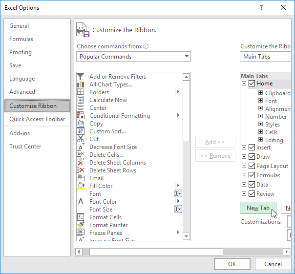
The essence of customizing the ribbon is mainly to add more command icons that are needed by the computer user.

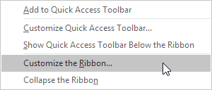
Step 1. Right click anywhere on the ribbon, and then click Customize the Ribbon.

Step 2. Click New Tab.

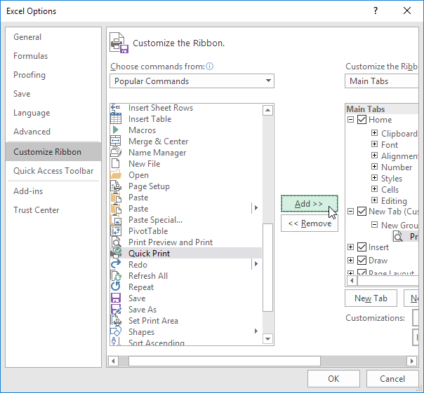
Step 3. Add the commands you like.

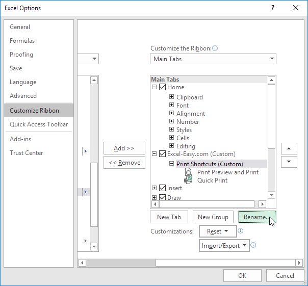
Step 4. Rename the tab and group.

You can easily create your own tab and add commands to it.

you can also add new groups to existing tabs. To hide a tab, uncheck the corresponding check box. Click Reset, Reset all customizations, to delete all Ribbon and Quick Access Toolbar customizations.

Collapse the Ribbon

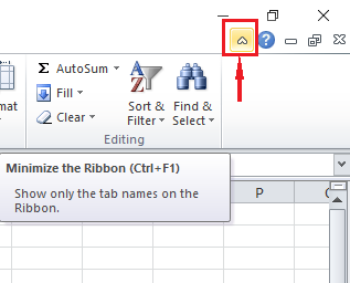
You can collapse the ribbon to get extra space on the screen.

There are 3 Ways to Collapse Ribbon in Excel

• Right click anywhere on the ribbon, and then click Collapse the Ribbon
• Using Excel Shortcut — press CTRL + F1
• Click the icon by the top most right as shown below: