Skip to content
Free Excel Tutorials
  • Home
  • Excel For Beginners
  • Excel Intermediate
  • Advanced Excel For Experts

Data Analysis

  • Create Scatter Chart in Excel
  • Conditional Formatting New Rule with Formulas in Excel
  • Conditional Formatting Rules in Excel
  • Chart Axes in Excel
  • How to calculate current stock or inventory in Excel

References

  • How to use Excel MMULT Function
  • CHOOSE function: Description, Usage, Syntax, Examples and Explanation
  • How to get address of first cell in range in Excel
  • Create hyperlink with VLOOKUP in Excel
  • How to get last column number in range in Excel

Data Validations

  • Excel Data validation whole percentage only
  • How To Create Drop-down List in Excel
  • Prevent invalid data entering in specific cells
  • Excel Data validation don’t exceed total
  • Excel Data validation number multiple 100

Change Cell Styles in Excel

by

Quickly format a cell by choosing a cell style.

Quickly format a range of cells by choosing a table style.

You can also create your own cell style.

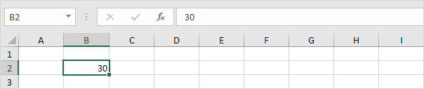
1. For example, select cell B2 below.

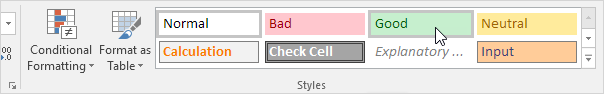
2. On the Home tab, in the Styles group, choose a cell style.
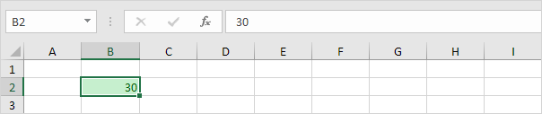
Result.

To create your own cell style, execute the following steps.

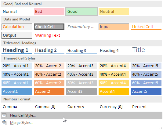
3. On the Home tab, in the Styles group, click the bottom right down arrow.

Here you can find many more cell styles.

4. Click New Cell Style.

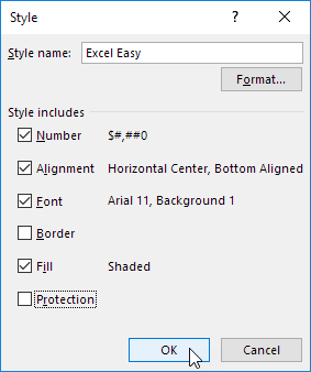
5. Enter a name and click the Format button to define the Number Format, Alignment, Font, Border, Fill and Protection of your cell style. Simply uncheck a check box if you don’t want to control this type of formatting.

6. Click OK.

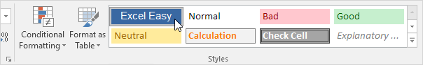
7. On the Home tab, in the Styles group, apply your own cell style.
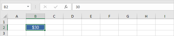
Result.

Note: right click a cell style to modify or delete it. Modifying a cell style affects all cells in a workbook that use that cell style. This can save a lot of time. A cell style is stored in the workbook where you create it. Open a new workbook and click on Merge Styles (under New Cell Style) to import a cell style (leave the old workbook with the cell style open).

Post navigation

Previous Post:

COSH function: Description, Usage, Syntax, Examples and Explanation

Next Post:

Excel Data validation require unique number

Leave a Reply Cancel reply

Your email address will not be published. Required fields are marked *

Learn Basic Excel

Ribbon
Workbook
Worksheets
Format Cells
Find & Select
Sort & Filter
Templates
Print
Share
Protect
Keyboard Shortcuts

Categories

  • Charts
  • Data Analysis
  • Data Validation
  • Excel Functions
    • Cube Functions
    • Database Functions
    • Date and Time Functions
    • Engineering Functions
    • Financial Functions
    • Information Functions
    • Logical Functions
    • Lookup and Reference Functions
    • Math and Trig Functions
    • Statistical Functions
    • Text Functions
    • Web Functions
  • Excel VBA
  • Excel Video Tutorials
  • Formatting
  • Grouping
  • Others

Logical Functions

  • TRUE function: Description, Usage, Syntax, Examples and Explanation
  • Check multiple cells are equal in Excel
  • How to use Excel AND Function
  • How to use Excel XOR Function
  • How to use Excel NOT Function

Date Time

  • How to calculate workdays per month in Excel
  • Convert Excel time to decimal seconds
  • Calculate total hours that fall between two times in Excel
  • WEEKNUM function: Description, Usage, Syntax, Examples and Explanation
  • Calculate time difference in hours as decimal value in Excel

Grouping

  • Map text to numbers in Excel
  • How to randomly assign data to groups in Excel
  • Map inputs to arbitrary values in Excel
  • Group numbers with VLOOKUP in Excel
  • Group numbers at uneven intervals in Excel

General

  • 231 Keyboard Shortcut Keys In Excel
  • How to test a range for numbers in Excel
  • Subtotal by color in Excel
  • How to count total number of cells in a rectangular range in Excel
  • How to calculate percent sold in Excel
© 2025 xlsoffice . All Right Reserved. | Teal Smiles | Abbreviations And Their Meaning