Skip to content
Free Excel Tutorials
  • Home
  • Excel For Beginners
  • Excel Intermediate
  • Advanced Excel For Experts

Data Analysis

  • How to Create One and Two Variable Data Tables in Excel
  • How to calculate correlation coefficient Correlation in Excel
  • How to Create Column Chart in Excel
  • How to Create Gantt Chart in Excel
  • How To Sort One Column or Multiple Columns in Excel

References

  • How to use Excel LOOKUP Function
  • How to get address of last cell in range in Excel
  • How to use Excel INDIRECT Function
  • How to get last row in mixed data with blanks in Excel
  • How to use Excel ROW Function

Data Validations

  • Excel Data validation no punctuation
  • Excel Data validation don’t exceed total
  • Excel Data validation exists in list
  • Excel Data validation allow weekday only
  • Prevent invalid data entering in specific cells

Average top 3 scores in Excel

by

This tutorial shows how to work  Average top 3 scores in Excel using the example below;

Formula

=AVERAGE(LARGE(range,{1,2,3}))

Explanation

To average the top 3 scores in a data set, you can use a formula based on the LARGE function.

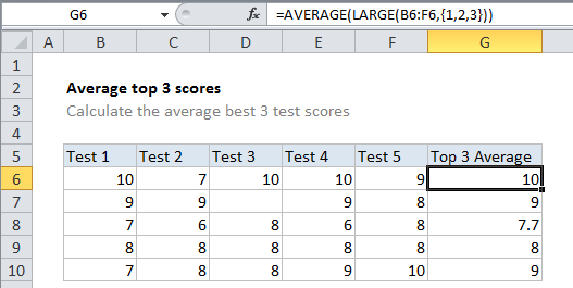
In the example shown, the formula in G6 is:

=AVERAGE(LARGE(B6:F6,{1,2,3}))

How this formula works

The LARGE function can retrieve the top nth value from a set of values. So, for example LARGE(A1:A10,1) will return highest value, LARGE(A1:A10,2) will return the 2nd highest value, and so on.

In this case, we are asking for more than one value by passing the array constant {1,2,3} into LARGE for the second argument. This causes LARGE to return an array result that includes the highest 3 values. The AVERAGE function then returns the average of these values.

The AVERAGE function is programmed to automatically handle array results, so it is not necessary to use Ctrl+Shift+Enter (CSE) to enter the formula.

Post navigation

Previous Post:

How to use Excel CHOOSE Function

Next Post:

Customize Ribbon In Excel

Leave a Reply Cancel reply

Your email address will not be published. Required fields are marked *

Learn Basic Excel

Ribbon
Workbook
Worksheets
Format Cells
Find & Select
Sort & Filter
Templates
Print
Share
Protect
Keyboard Shortcuts

Categories

  • Charts
  • Data Analysis
  • Data Validation
  • Excel Functions
    • Cube Functions
    • Database Functions
    • Date and Time Functions
    • Engineering Functions
    • Financial Functions
    • Information Functions
    • Logical Functions
    • Lookup and Reference Functions
    • Math and Trig Functions
    • Statistical Functions
    • Text Functions
    • Web Functions
  • Excel VBA
  • Excel Video Tutorials
  • Formatting
  • Grouping
  • Others

Logical Functions

  • Invoice status with nested if in Excel
  • NOT function: Description, Usage, Syntax, Examples and Explanation
  • IF with boolean logic in Excel
  • IFNA function: Description, Usage, Syntax, Examples and Explanation
  • How to use Excel AND Function

Date Time

  • Convert date to Julian format in Excel
  • Calculate time difference in hours as decimal value in Excel
  • Two ways to sum time over 30 minutes in Excel
  • Add months to date in Excel
  • DATE function: Description, Usage, Syntax, Examples and Explanation

Grouping

  • Group numbers with VLOOKUP in Excel
  • Map text to numbers in Excel
  • Group times into 3 hour buckets in Excel
  • Group numbers at uneven intervals in Excel
  • Calculate conditional mode with criteria in Excel

General

  • Check if range contains a value not in another range in Excel
  • How to get amount with percentage in Excel
  • How to calculate project complete percentage in Excel
  • Transpose: Switch ‘Rows to Columns’ or ‘Columns to Rows’ in Excel
  • How to choose page/paper size in Excel before Printing
© 2025 xlsoffice . All Right Reserved. | Teal Smiles | Abbreviations And Their Meaning