Highlight cells that begin with in Excel

Explanation

Note: Excel contains many built-in “presets” for highlighting values with conditional formatting, including a preset to highlight cells that begin with specific text. However, if you want more flexibility, you can use your own formula, as explained in this article.

If you want to highlight cells that begin with certain text, you can use a simple formula that returns TRUE when a cell starts with the text (substring) you specify.

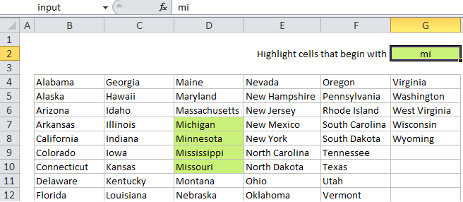
For example, if you want to highlight any cells in the range B4:G12 that start with “mi”, you can use:

=SEARCH("mi",B4)=1

Note: with conditional formatting, it’s important that the formula be entered relative to the “active cell” in the selection, which is assumed to be B4 in this case.

How this formula works

When you use a formula to apply conditional formatting, the formula is evaluated relative to the active cell in the selection at the time the rule is created. In this case, the rule is evaluated for each cell in B4:G12, and B4 will change to the address of the cell being evaluated each time, since it is entered as a relative address.

The formula itself uses the SEARCH function to match cells that begin with “mi”. SEARCH returns a number that indicates position when the text is found, and a #VALUE! error if not. When SEARCH returns the number 1, we know that the cell value begins with “mi”. The formula returns TRUE when the position is 1 and FALSE for any other value (including errors).

With a named input cell

If you use a named range to name an input cell (i.e. name G2 “input”), you can simply for the formula and make a much more flexible rule:

=SEARCH(input,B4)=1

Then when you change the value in “input”, the conditional formatting will instantly be updated.

Case sensitive option

SEARCH is not case-sensitive, so if you need to check case as well, you can use the FIND function instead:

=FIND(input,B4)=1

The FIND function works like SEARCH, but is case-sensitive.