Skip to content
xlsoffice. All Rights Reserved
  • Home
  • Excel For Beginners
  • Excel Intermediate
  • Advanced Excel For Experts

Lookup and Reference Examples

  • How to use Excel ROW Function
  • Two-way lookup with VLOOKUP in Excel
  • Left Lookup in Excel
  • Find Closest Match in Excel Using INDEX, MATCH, ABS and MIN functions
  • How to use Excel VLOOKUP Function

Data Analysis Examples

  • Chart Axes in Excel
  • Randomize/ Shuffle List in Excel
  • Excel Frequency Function Example
  • Move chart to a separate worksheet in Excel
  • Managing Conditional Formatting Rules in Excel

Data Validation Examples

  • Excel Data validation don’t exceed total
  • Excel Data validation exists in list
  • Excel Data validation must not contain
  • Excel Data validation unique values only
  • Excel Data validation must begin with

How to test for all values in a range are at least in Excel

by

To test if all values in a range are at least a certain threshold value, you can use the COUNTIF function together with the NOT function.

Formula

=NOT(COUNTIF(range,"<65"))

Explanation

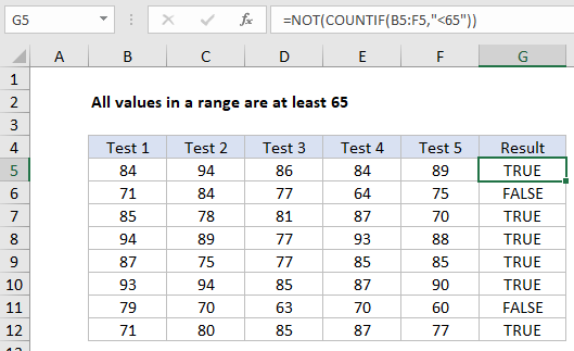
In the example shown, the formula in G5 is:

=NOT(COUNTIF(B5:F5,"<65"))

How this formula works

At the core, this formula uses the COUNTIF function to count any cells that fall below a given value, which is hardcoded as 65 in the formula:

COUNTIF(B5:F5,"<65")

In this part of the formula, COUNTIF will return a positive number if any cell in the range is less than 65, and zero if not. In the range B5:F5, there is one score below 65 so COUNTIF will return 1.

Worked Example:   Count cells greater than in Excel

The NOT function is used to convert the number of from COUNTIF into a TRUE or FALSE result. The trick is that NOT also “flips” the result at the same time:

  • If any values are less than 65, COUNTIF returns a positive number and NOT returns FALSE
  • f no values are less than 65, COUNTIF returns a zero and NOT returns TRUE
Worked Example:   Running count of occurrence in list in Excel

This is the equivalent of wrapping COUNTIF inside IF and providing a “reversed” TRUE and FALSE result like this:

=IF(COUNTIF(B5:F5,"<65"),FALSE,TRUE)

Post navigation

Previous Post:

How to get address of last cell in range in Excel

Next Post:

How to get relative column numbers in a range in Excel

Leave a Reply Cancel reply

Your email address will not be published. Required fields are marked *

Learn Basic Excel

Ribbon
Workbook
Worksheets
Format Cells
Find & Select
Sort & Filter
Templates
Print
Share
Protect
Keyboard Shortcuts

Categories

  • Charts
  • Data Analysis
  • Data Validation
  • Excel Functions
    • Cube Functions
    • Database Functions
    • Date and Time Functions
    • Engineering Functions
    • Financial Functions
    • Information Functions
    • Logical Functions
    • Lookup and Reference Functions
    • Math and Trig Functions
    • Statistical Functions
    • Text Functions
    • Web Functions
  • Excel VBA
  • Excel Video Tutorials
  • Formatting
  • Grouping
  • Others
  • How to extract name from email address in Excel
  • Complete List of Excel Text Functions References and Examples
  • How to count line breaks in cell in Excel worksheet
  • How to check if cell contains some words but not others in Excel
  • How to get page from URL in Excel
  • Steps to create Dynamic calendar grid in Excel
  • Next biweekly payday from date in Excel
  • Custom weekday abbreviation in Excel
  • EOMONTH function: Description, Usage, Syntax, Examples and Explanation
  • Convert Excel time to Unix time in Excel
  • NPER function: Description, Usage, Syntax, Examples and Explanation
  • DURATION function: Description, Usage, Syntax, Examples and Explanation
  • PMT, RATE, NPER, PV and FV Financial Functions in Excel
  • How to calculate annual compound interest schedule in Excel
  • PRICEDISC function: Description, Usage, Syntax, Examples and Explanation
© 2022 xlsoffice . All Right Reserved. | Teal Smiles