Count visible rows only with criteria in Excel

This tutorial shows how to Count visible rows only with criteria in Excel using the example below;

Formula

=SUMPRODUCT((range=criteria)*(SUBTOTAL(3,OFFSET(range,rows,0,1))))

Explanation

To count visible rows only with criteria, you can use a rather complex formula based on SUMPRODUCT, SUBTOTAL, and OFFSET.

The problem

The SUBTOTAL function can easily generate sums and counts for hidden and non-hidden rows. However, it isn’t able to handle criteria (i.e. like COUNTIF or SUMIF).

The solution

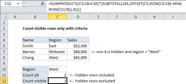
The solution is to use SUMPRODUCT to apply both the SUBTOTAL function (via OFFSET) and the criteria. In the example shown, the formula in C12 is:

=SUMPRODUCT((C5:C8=C10)*(SUBTOTAL(103,OFFSET(C5,ROW(C5:C8)-MIN(ROW(C5:C8)),0))))

How this formula works

The core of this formula is the array calculations inside of SUMPRODUCT. The first array applies the criteria, and the second array handles the “visibility problem”.

=SUMPRODUCT(criteria*visibility)

The criteria is applied with part of the formula:

=(C5:C8=C10)

Which generates an array like this:

{FALSE;TRUE;FALSE;TRUE}

Where TRUE means “meets criteria”. Note that because we are using multiplication (*) inside the first (and only) array given to SUMPRODUCT, the TRUE FALSE values will automatically be converted to:

{0;1;0;1}

The visibility filter is applied using SUBTOTAL.

SUBTOTAL is able to exclude hidden rows in a variety of calculations, so we can use it in this case to generate a “filter” to exclude hidden rows inside of SUMPRODUCT. The problem though is that SUBTOTAL returns a single number, while we need an array to use it successfully inside SUMPRODUCT.

The trick is to use OFFSET to feed SUBTOTAL one reference per row, so that OFFSET will return one result per row.

Of course, that requires another trick, which is to give OFFSET an array that contains one number per row, starting with zero. We do that using:

=ROW(C5:C8)-MIN(ROW(C5:C8)

Which will generate an array like this:

{0;1;2;3}

So, the second array, which handles visibility using SUBTOTAL, is generated like this:

=SUBTOTAL(103,OFFSET(C5,ROW(C5:C8)-MIN(ROW(C5:C8)),0))
=SUBTOTAL(103,OFFSET(C5,{0;1;2;3},0))
=SUBTOTAL(103,{"East";"West";"Midwest";"West"})
={1;0;1;1}

And, finally, we have:

=SUMPRODUCT({0,1,0,1}*{1;0;1;1})

Which returns 1.

Multiple criteria

You can extend the formula to handle multiple criteria like this:

=SUMPRODUCT((range1=criteria1)*(range2=criteria2)*(SUBTOTAL(3,OFFSET(range,rows,0,1))))