
Skip to content
Free Excel Tutorials
  • Home
  • Excel For Beginners
  • Excel Intermediate
  • Advanced Excel For Experts

Data Analysis

  • Error Bars in Excel
  • How to do a t-Test in Excel?
  • How to create a Histogram in Excel
  • Conditional Formatting Data bars Examples in Excel
  • Randomize/ Shuffle List in Excel

References

  • Extract all partial matches in Excel
  • Find closest match in Excel
  • How to get relative row numbers in a range in Excel
  • How to retrieve first match between two ranges in Excel
  • How to use Excel ROW Function

Data Validations

  • Excel Data validation allow uppercase only
  • Excel Data validation date in specific year
  • Excel Data validation with conditional list
  • Excel Data validation whole percentage only
  • Excel Data validation don’t exceed total

Calculate a ratio from two numbers in Excel

by

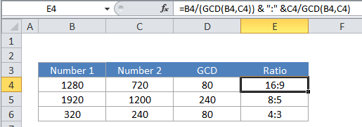
To generate the ratio of two numbers to each other (e.g. 4:3, 16:9, etc.), you can do using division, the GCD function, and concatenation. In the formula  of the formula below num1 represents the first number (the antecedent) and num2 represents the second number (the consequent).

Formula

=num1/GCD(num1,num2)&":"&num2/GCD(num1,num2)
Explanation

In the example, the active cell contains this formula:

=B4/GCD(B4,C4)&":"&C4/GCD(B4,C4)

Note: the GCD function only works with integers.

How this formula works

This formula looks complicated, but, at the core, it is quite simple, and created in two parts like so:

= (formula for number1) &":"& (formula for number2)

On the left, the GCD function is used to calculated the greatest common divisor (GCD) of the two numbers. Then the first number is divided by the GCD. On the right, the same operations are performed with the second number.

Next, the result of the right and left operations are joined together using concatenation, with the colon (“:”) as a separator. So, altogether, we have:

=B4/(GCD(B4,C4)) &":"& C4/GCD(B4,C4)
=1280/(GCD(1280,720)) &":"& 720/GCD(1280,720)
=1280/80 &":"& 720/80
=16 &":"& 9
=16:9

Note that the final result of this formula is a text value.

Post navigation

Previous Post:

How to calculate project complete percentage in Excel

Next Post:

Popularly Used Excel Functions and their examples

Leave a Reply Cancel reply

Your email address will not be published. Required fields are marked *

Learn Basic Excel

Ribbon
Workbook
Worksheets
Format Cells
Find & Select
Sort & Filter
Templates
Print
Share
Protect
Keyboard Shortcuts

Categories

  • Charts
  • Data Analysis
  • Data Validation
  • Excel Functions
    • Cube Functions
    • Database Functions
    • Date and Time Functions
    • Engineering Functions
    • Financial Functions
    • Information Functions
    • Logical Functions
    • Lookup and Reference Functions
    • Math and Trig Functions
    • Statistical Functions
    • Text Functions
    • Web Functions
  • Excel VBA
  • Excel Video Tutorials
  • Formatting
  • Grouping
  • Others

Logical Functions

  • Invoice status with nested if in Excel
  • How to use Excel TRUE Function
  • Nested IF function example in Excel
  • AND function: Description, Usage, Syntax, Examples and Explanation
  • How to return blank in place of #DIV/0! error in Excel

Date Time

  • Add months to date in Excel
  • TIME function: Description, Usage, Syntax, Examples and Explanation
  • Steps to create Dynamic calendar grid in Excel
  • DAYS360 function: Description, Usage, Syntax, Examples and Explanation
  • Custom weekday abbreviation in Excel

Grouping

  • Group times into 3 hour buckets in Excel
  • Group arbitrary text values in Excel
  • Group times into unequal buckets in Excel
  • How to randomly assign people to groups in Excel
  • Calculate conditional mode with criteria in Excel

General

  • How to create dynamic worksheet reference in Excel
  • Lock Cells in a Worksheet Excel
  • How to Create Calendar in Excel
  • Count cells that do not contain many strings in Excel
  • How to password protect excel sheet?
© 2026 xlsoffice . All Right Reserved. | Teal Smiles | Abbreviations And Their Meaning