How to get address of named range in Excel

To get the full address of a named range with an Excel formula, you can use the ADDRESS function together with the ROW and COLUMN functions.

Formula

=ADDRESS(ROW(nr),COLUMN(nr))&":
"&ADDRESS(ROW(nr)+ROWS(nr)-1,
COLUMN(nr)+COLUMNS(nr)-1)

Explanation

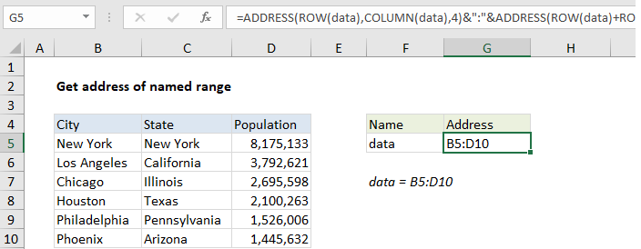
In the example shown, the formula in G5 is:

=ADDRESS(ROW(data),COLUMN(data),4)
&":"&ADDRESS(ROW(data)+ROWS
(data)-1,COLUMN(data)+COLUMNS(data)-1,4)

where “data” is the named range B5:D10

How this formula works

The core of this formula is the ADDRESS function, which is used to return a cell address based on a given row and column. Unfortunately, the formula gets somewhat complicated because we need to use ADDRESS twice: once to get address of the first cell in the range, and once to get the address of the last cell in the range. The two results are joined with concatenation and the range operator (:) and the full range is returned as text.

To get the first cell in the range, we use this expression:

=ADDRESS(ROW(data),COLUMN(data))

ROW returns the first row number associated with the range, 5*.

COLUMN returns the first column number associated with the range, 2.

With abs_num set to 4 (relative), ADDRESS returns the text “B5”.

=ADDRESS(5,2,4) // returns "B5"

To get the last cell in the range, we use this expression:

=ADDRESS(ROW(data)+ROWS(data)-1,
COLUMN(data)+COLUMNS(data)-1,4)

See this page for a detailed explanation.

Essentially, we follow the same idea as above, adding simple math to calculate the last row and last column of the range, which are fed as before into ADDRESS with abs_num set to 4. This reduces to the following expression, which returns the text “D10”:

=ADDRESS(10,4,4) // returns "D10"

Both results are concatenated with a colon to get a final range address as text:

="B5"&":"&"D10"
="B5:D10

Named range from another cell

To get an address for a named range in another cell, you’ll need to use the INDIRECT function. For example, to get the address of a name in A1, you would use:

=ADDRESS(ROW(INDIRECT(A1)),COLUMN(INDIRECT
(A1)))&":"&ADDRESS(ROW(INDIRECT(A1))+ROWS
(INDIRECT(A1))-1,COLUMN(INDIRECT(A1))
+COLUMNS(INDIRECT(A1))-1)

Set abs_num to 4 inside ADDRESS to get a relative address.

* Actually, in all cases where we use ROW and COLUMN with a multi-cell named range, we’ll get back an array of numbers instead of a single value. However, since we aren’t using an array formula, processing is limited to the first item in these arrays.