Skip to content
Free Excel Tutorials
  • Home
  • Excel For Beginners
  • Excel Intermediate
  • Advanced Excel For Experts

Data Analysis

  • How to calculate correlation coefficient Correlation in Excel
  • Conditional Formatting New Rule with Formulas in Excel
  • Excel Pie Chart
  • How To Create Frequency Distribution in Excel
  • Chart Axes in Excel

References

  • Merge tables with VLOOKUP in Excel
  • Offset in Excel
  • Create hyperlink with VLOOKUP in Excel
  • Approximate match with multiple criteria in Excel
  • How to use Excel INDIRECT Function

Data Validations

  • Excel Data validation with conditional list
  • Excel Data validation must not contain
  • Data validation must not exist in list
  • Excel Data validation date in specific year
  • Excel Data validation only dates between

How to create dynamic named range with OFFSET in Excel

by

One way to create a dynamic named range with a formula is to use the OFFSET function together with the COUNTA function. Dynamic ranges are also known as expanding ranges – they automatically expand and contract  to accommodate new or deleted data.

Note: OFFSET is a volatile function, which means it recalculates with every change to a worksheet. With a modern machine and smaller data set, this should’t cause a problem but you may see slower performance on large data sets. In that case, consider building a dynamic named range with the INDEX function instead.

Formula

=OFFSET(origin,0,0,COUNTA(range),COUNTA(range))

Explanation

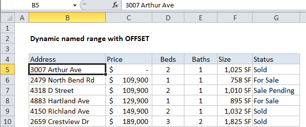
In the example shown, the formula used for the dynamic range is:

=OFFSET(B5,0,0,COUNTA($B$5:$B$100),COUNTA($B$4:$Z$4))

How this formula works

This formula uses the OFFSET function to generate a range that expands and contracts by adjusting height and width based on a count of non-empty cells.

The first argument in OFFSET represents the first cell in the data (the origin), which in this case is cell B5. The next two arguments are offsets for rows and columns, and are supplied as zero.

The last two arguments represent height and width. Height and width are generated on the fly by using COUNTA, which makes the the resulting reference dynamic.

For height, we use the COUNTA function to count non-empty values in the range B5:B100. This assumes no blank values in the data, and no values beyond B100. COUNTA returns 6.

For width, we use the COUNTA function to count non-empty values in the range B5:Z5. This assumes no header cells, and no headers beyond Z5. COUNTA returns 6.

At this point, the formula looks like this:

=OFFSET(B5,0,0,6,6)

With this information, OFFSET returns a reference to B5:G10, which corresponds to a range 6 rows height by 6 columns across.

Note: The ranges used for height and width should be adjusted to match the worksheet layout.

Variation with full column/row references

You can also use full column and row references for height and width like so:

=OFFSET($B$5,0,0,COUNTA($B:$B)-2,COUNTA($4:$4))

Note that height is being adjusted with -2 to take into account header and title values in cells B4 and B2. The advantage to this approach is the simplicity of the ranges inside COUNTA. The disadvantage comes from the huge size full columns and rows — care must be taken to prevent errant values outside the range, as they can easily throw off the count.

Post navigation

Previous Post:

How to calculate project complete percentage in Excel

Next Post:

Popularly Used Excel Functions and their examples

Leave a Reply Cancel reply

Your email address will not be published. Required fields are marked *

Learn Basic Excel

Ribbon
Workbook
Worksheets
Format Cells
Find & Select
Sort & Filter
Templates
Print
Share
Protect
Keyboard Shortcuts

Categories

  • Charts
  • Data Analysis
  • Data Validation
  • Excel Functions
    • Cube Functions
    • Database Functions
    • Date and Time Functions
    • Engineering Functions
    • Financial Functions
    • Information Functions
    • Logical Functions
    • Lookup and Reference Functions
    • Math and Trig Functions
    • Statistical Functions
    • Text Functions
    • Web Functions
  • Excel VBA
  • Excel Video Tutorials
  • Formatting
  • Grouping
  • Others

Logical Functions

  • FALSE function: Description, Usage, Syntax, Examples and Explanation
  • IFERROR function: Description, Usage, Syntax, Examples and Explanation
  • NOT function: Description, Usage, Syntax, Examples and Explanation
  • How to use Excel TRUE Function
  • TRUE function: Description, Usage, Syntax, Examples and Explanation

Date Time

  • WEEKDAY function: Description, Usage, Syntax, Examples and Explanation
  • Get first day of month in Excel
  • YEARFRAC function: Description, Usage, Syntax, Examples and Explanation
  • How to calculate Day of the Year in Excel
  • DAY function: Description, Usage, Syntax, Examples and Explanation

Grouping

  • Group times into 3 hour buckets in Excel
  • Group numbers with VLOOKUP in Excel
  • Categorize text with keywords in Excel
  • If cell contains one of many things in Excel
  • Group numbers at uneven intervals in Excel

General

  • Index and match on multiple columns in Excel
  • How to create dynamic named range with INDEX in Excel
  • How to calculate percentage of total in Excel
  • How to calculate profit margin percentage in Excel
  • How to get random value from list or table in Excel
© 2026 xlsoffice . All Right Reserved. | Teal Smiles | Abbreviations And Their Meaning