How to Calculate Tax Rates in Excel

This example teaches you how to calculate the tax on an income using the VLOOKUP function in Excel. The following tax rates apply to individuals who are residents of Australia.

Taxable income	Tax on this income
0 – $18,200	Nil
$18,201 – $37,000	19c for each $1 over $18,200
$37,001 – $87,000	$3,572 plus 32.5c for each $1 over $37,000
$87,001 – $180,000	$19,822 plus 37c for each $1 over $87,000
$180,001 and over	$54,232 plus 45c for each $1 over $180,000

Example: if income is 39000, tax equals 3572 + 0.325 * (39000 – 37000) = 3572 + 650 = $4222

To automatically calculate the tax on an income, execute the following steps.

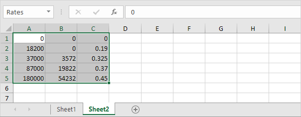
1. On the second sheet, create the following range and name it Rates.

2. When you set the fourth argument of the VLOOKUP function to TRUE, the VLOOKUP function returns an exact match or if not found, it returns the largest value smaller than lookup_value (A2). That’s exactly what we want!

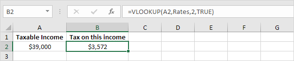
Explanation: Excel cannot find 39000 in the first column of Rates. However, it can find 37000 (the largest value smaller than 39000). As a result, it returns 3572 (col_index_num, the third argument, is set to 2).

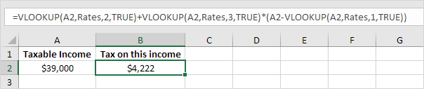
3. Now, what’s left is the remainder of the equation, + 0.325 * (39000 – 37000). This is easy. We can return 0.325 by setting col_index_num to 3 and return 37000 by setting col_index_num to 1. The complete formula below does the trick.

Note: when you set the fourth argument of the VLOOKUP function to TRUE, the first column of the table must be sorted in ascending order.