Color Scales in Excel make it very easy to visualize values in a range of cells. The shade of the color represents the value in the cell.

To add a color scale, execute the following steps.

1. Select a range.

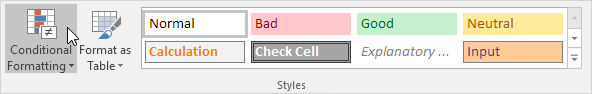
2. On the Home tab, in the Styles group, click Conditional Formatting.

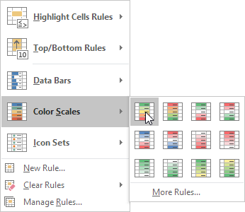
3. Click Color Scales and click a subtype.

Result:

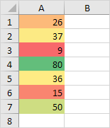
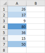
Explanation: by default, for 3-Color scales, Excel calculates the 50th percentile (also known as median, middle value or midpoint). The cell that holds the minimum value (9) is colored red. The cell that holds the median (36) is colored yellow, and the cell that holds the maximum value (80) is colored green. All other cells are colored proportionally.

Read on to further customize this color scale.

4. Select the range A1:A7.

5. On the Home tab, in the Styles group, click Conditional Formatting, Manage Rules.

6. Click Edit rule.

Excel launches the Edit Formatting Rule dialog box. Here you can further customize your color scale (Format Style, Minimum, Midpoint and Maximum, Color, etc).

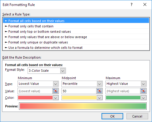
Note: to directly launch this dialog box for new rules, at step 3, click More Rules.

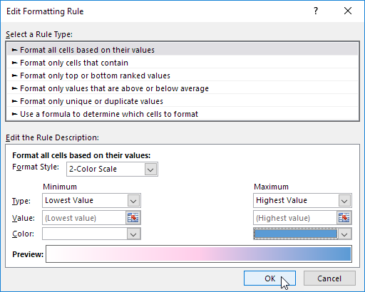
7. Select 2-Color Scale from the Format Style drop-down list and select white and blue.

8. Click OK twice.

Result.