Skip to content
Free Excel Tutorials
  • Home
  • Excel For Beginners
  • Excel Intermediate
  • Advanced Excel For Experts

Data Analysis

  • Get column name from index in Excel Table
  • Calculate Conditional Percentile ‘IF’ in table in Excel
  • Get column index in Excel Table
  • Conditional Formatting Icon Sets Examples in Excel
  • How to create running total in an Excel Table

References

  • LOOKUP function: Description, Usage, Syntax, Examples and Explanation
  • How to get last row in mixed data with blanks in Excel
  • How to retrieve first match between two ranges in Excel
  • Create hyperlink with VLOOKUP in Excel
  • How to get last column number in range in Excel

Data Validations

  • Excel Data validation date in next 30 days
  • Excel Data validation with conditional list
  • Excel Data validation number multiple 100
  • Excel Data validation only dates between
  • Excel Data validation require unique number

Cash denomination calculator in Excel

by

To calculate required currency denominations, given a specific amount, you can build a currency calculation table as shown in the example. This solution uses the INT and SUMPRODUCT functions.

Formula

=INT((amount-SUMPRODUCT(denoms,counts))/currentdenom)

Cash denomination calculator in Excel

Explanation

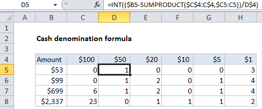
In the example show, the formula in D5 is:

=INT(($B5-SUMPRODUCT($C$4:C$4,$C5:C5))/D$4)

How this formula works

To start off, the formula in C5 is:

=INT($B5/C$4)

This formula divides the amount in column B by the denomination in C4 (100) and discards the remainder using the INT function. The formulas in column C are simpler than those in the next several columns because this is the first denomination – we don’t need to worry about previous counts.

Next in D5 we first figure out what the value of existing denomination counts with:

SUMPRODUCT($C$4:C$4,$C5:C5)

Here SUMPRODUCT is configured with two arrays, both configured carefully.

Array1 consists of denominations from row 4. This range is carefully constructed to be “expand” when copied across the table to the right. The first reference is absolute ($C$4) and the second reference is “mixed” (C$4) – the row is locked but the column will change, causing the range to expand.

Array2 consists of existing denomination counts from row 5, with the same approach as above. The range will expand as it’s copied to the right.

The result of this SUMPRODUCT operation is the total value of existing denomination counts so far in the table. This is subtracted from the original value in column B, then divided by the “current” denomination from row 4. As before, we use INT to remove any remainder.

As the formulas in column C are copied across the table, the correct counts for each denomination are calculated.

Checking the result

If you want to check your results, add a column to the end of the table with a formula like this:

=SUMPRODUCT(C$4:H$4,C5:H5)

In each row, SUMPRODUCT multiplies all counts by all denominations and returns a result that should match the original values in column B.

Post navigation

Previous Post:

How to calculate project complete percentage in Excel

Next Post:

Popularly Used Excel Functions and their examples

Leave a Reply Cancel reply

Your email address will not be published. Required fields are marked *

Learn Basic Excel

Ribbon
Workbook
Worksheets
Format Cells
Find & Select
Sort & Filter
Templates
Print
Share
Protect
Keyboard Shortcuts

Categories

  • Charts
  • Data Analysis
  • Data Validation
  • Excel Functions
    • Cube Functions
    • Database Functions
    • Date and Time Functions
    • Engineering Functions
    • Financial Functions
    • Information Functions
    • Logical Functions
    • Lookup and Reference Functions
    • Math and Trig Functions
    • Statistical Functions
    • Text Functions
    • Web Functions
  • Excel VBA
  • Excel Video Tutorials
  • Formatting
  • Grouping
  • Others

Logical Functions

  • XOR function: Description, Usage, Syntax, Examples and Explanation
  • IFNA function: Description, Usage, Syntax, Examples and Explanation
  • How to return blank in place of #DIV/0! error in Excel
  • IFERROR function: Description, Usage, Syntax, Examples and Explanation
  • How to use IFS function in Excel

Date Time

  • EOMONTH function: Description, Usage, Syntax, Examples and Explanation
  • Get day name from date in Excel
  • How to join date and text together in Excel
  • Get days between dates ignoring years in Excel
  • Get month name from date in Excel

Grouping

  • Running count group by n size in Excel
  • How to randomly assign people to groups in Excel
  • If cell contains one of many things in Excel
  • Map inputs to arbitrary values in Excel
  • Group times into 3 hour buckets in Excel

General

  • 3D SUMIF for multiple worksheets in Excel
  • Count cells that do not contain many strings in Excel
  • Excel Ribbon Quick Overview For Beginners
  • Check if multiple cells have same value with case sensitive in Excel
  • Creating and Opening an existing file in Excel
© 2025 xlsoffice . All Right Reserved. | Teal Smiles | Abbreviations And Their Meaning