Calculate interest rate for loan in Excel

To calculate the periodic interest rate for a loan, given the loan amount, the number of payment periods, and the payment amount, you can use the RATE function.

Formula

=RATE(periods,payment,-amount)*12

Explanation

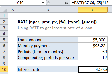
In the example shown, the formula in C10 is:

=RATE(C7,C6,-C5)*12

Loans have four primary components: the amount, the interest rate, the number of periodic payments (the loan term) and a payment amount per period. One use of the RATE function is to calculate the periodic interest rate when the amount, number of payment periods, and payment amount are known.

For this example, we want to calculate the interest rate for  $5000 loan, and with 60 payments of $93.22 each. The NPER function is configured as follows:

NPER – The number of periods is 60, and comes from C7.

pmt – The payment is $93.22, and comes from cell C7.

pv – The present value is $5000, and comes from C5. The amount is input as a negative value by adding a negative sign in from of C5:

-C5

With these inputs, the RATE function returns .38%, which is the periodic interest rate. To get an annual interest rate, this result is multiplied by 12:

=RATE(C7,C6,-C5)*12