How to convert text string to array in Excel

To convert a string to an array that contains one item for each letter, you can use an array formula based on the MID, ROW, LEN and INDIRECT functions. This can sometimes be useful inside other formulas that manipulate text at the character level.

 Formula

{=MID(string,ROW(INDIRECT("1:"&LEN(string))),1)}

Note: this is an array formula and must be entered with control + shift + enter.

Explanation

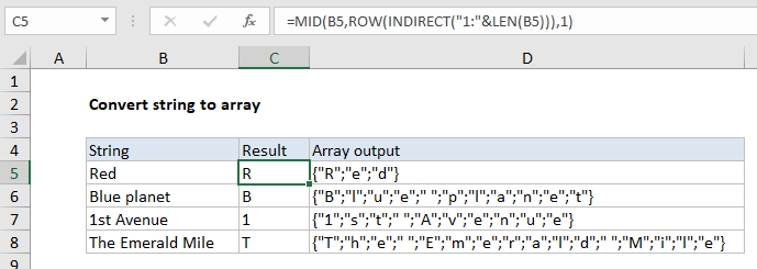
In the example shown, the formula in C5 is:

{=MID(B5,ROW(INDIRECT("1:"&LEN(B5))),1)}

How this formula works

Working from the inside out, the LEN function calculates the length of the string, and this is joined by concatenation to “1:”, creating a text range like this: “1:3”

This text is passed into INDIRECT, which evaluates the text as a reference and returns the result to the ROW function. The ROW function returns the rows contained in the reference in an array of numbers like this:

{1;2;3}

Notice we have one number for each letter in the original text.

This array goes into the MID function, for the start_num argument. The text comes from column B, and the number of characters is hardcoded as 1

Finally, with multiple start numbers, MID returns multiple results in an array like this.

{"R";"e";"d"}