How to check if cell contains one of many things in Excel

Context

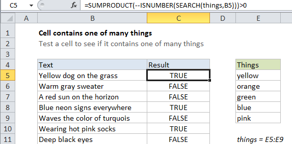
Let’s say you have a list of text strings in the range B5:B11, and you want to test each cell against another list of things in the named range “things” E5:E9. In other words, for each cell in B5:B11, you want to know: does this cell contain any of the things in E5:E9?

You could start build a big formula based on nested IF statements, but that won’t be any fun at all, especially if the list of things you want to check for is large.

Solution

The solution is to to create a formula that can test for multiple values and return a list of TRUE / FALSE values. Once we have that, we can process that list (an array, actually) with SUMPRODUCT.

The formula we’re using looks like this:

=SUMPRODUCT(--ISNUMBER(SEARCH(things,B5)))>0

How this formula works

The key is this snippet:

ISNUMBER(SEARCH(things,B5))

This is based on another formula (explained in detail here) that simply checks a cell for a single substring. If the cell contains the substring, the formula returns TRUE. If not, the formula returns FALSE.

However, if we give the same formula a list of things (in this case, we are using a named range called “things”, E5:E11) it will give us back a list of TRUE / FALSE values. The result is actually an array that looks like this:

{TRUE;FALSE;FALSE;FALSE;FALSE}

Notice that if we have even one TRUE in the array, we know a cell contains at least one thing in the list. So, we can force the TRUE / FALSE values to 1s and 0s with a double negative (–, also called a double unary):

--ISNUMBER(SEARCH(things,B5))

which yields an array like this:

{1;0;0;0;0}

Now we process the result with SUMPRODUCT, which will add up the entire array. We know if we get a non-zero result, we have a “hit”, so we use >0 to force a final result of either TRUE or FALSE.

=SUMPRODUCT(--ISNUMBER(SEARCH(things,B5)))>0

With a hard-coded list

There’s no requirement that you use a range for your list of things. If you’re only looking for a small number of things, you can use a list in array format, which is called an array constant. For example, if you’re just looking for the colors red, blue, and green, you can use {“red”,”blue”,”green”} like this:

=SUMPRODUCT(--ISNUMBER(SEARCH({"red","blue","green"},B5)))>0

Preventing false matches

One problem with this approach is you may get false matches from substrings that appear inside longer words. For example, if you try to match “dr” you may also find “Andrea”, “drink”, “dry”, etc. since “dr” appears inside these words. This happens because SEARCH automatically does a “contains” match.

For a quick hack, you can add space around the search words (i.e. ” dr “, or “dr “) to avoid catching “dr” in another word. But this will fail if “dr” appears first or last in a cell, or appears with punctuation.

If you need a more accurate solution, one option is to normalize the text first in a helper column, taking care to also add a leading and trailing space. Then you use the formula on this page on the resulting text.