Skip to content
Free Excel Tutorials
  • Home
  • Excel For Beginners
  • Excel Intermediate
  • Advanced Excel For Experts

Data Analysis

  • How to conditionally sum numeric data in an Excel table using SUMIFS
  • How to Create One and Two Variable Data Tables in Excel
  • Subtotal function in Excel
  • Conditional Formatting Data bars Examples in Excel
  • Calculate Conditional Percentile ‘IF’ in table in Excel

References

  • How to retrieve first match between two ranges in Excel
  • How to use Excel TRANSPOSE Function
  • Extract all partial matches in Excel
  • LOOKUP function: Description, Usage, Syntax, Examples and Explanation
  • Count rows that contain specific values in Excel

Data Validations

  • Excel Data validation with conditional list
  • Excel Data validation allow uppercase only
  • Excel Data validation date in next 30 days
  • Data validation must not exist in list
  • Excel Data validation unique values only

How to abbreviate names or words in Excel

by

To abbreviate text that contains capital letters, you can try this array formula based on the TEXTJOIN function, which is new in Excel 2016. You can use this approach to create initials from names, or to create acronyms. Only capital letters will survive this formula, so the source text must include capitalized words. You can use the PROPER function to capitalize words if needed. See example below;

 Formula

=TEXTJOIN("",1,IF(ISNUMBER(MATCH(CODE(MID(A1,ROW(INDIRECT("1:"&LEN(A1))),1)),ROW(INDIRECT("63:90")),0)),MID(A1,ROW(INDIRECT("1:"&LEN(A1))),1),""))

How to abbreviate names or words in Excel

Explanation

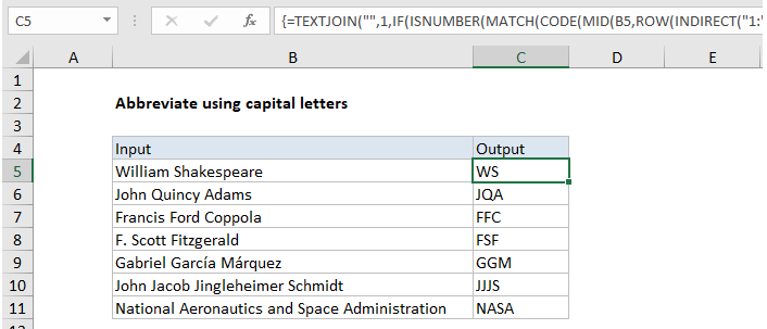
In the example shown, the formula in C5 is:

=TEXTJOIN("",1,IF(ISNUMBER(MATCH(CODE(MID(B5,ROW(INDIRECT("1:"&LEN(B5))),1)),ROW(INDIRECT("63:90")),0)),MID(B5,ROW(INDIRECT("1:"&LEN(B5))),1),""))

How this formula works

Working from the inside out, the MID function is used to cast the string into an array of individual letters:

MID(B5,ROW(INDIRECT("1:"&LEN(B5))),1)

In this part of the formula, MID, ROW, INDIRECT, and LEN are used to convert a string to an array or letters, as described here.

MID returns an array of all characters in the text.

{“W”;”i”;”l”;”l”;”i”;”a”;”m”;” “;”S”;”h”;”a”;”k”;”e”;”s”;”p”;”e”;”a”;”r”;”e”}

This array is fed into the CODE function, which outputs an array of numeric ascii codes, one for each letter.

Separately, ROW and INDIRECT are used to create another numeric array:

ROW(INDIRECT("63:90")

This is the clever bit. The numbers 63 to 90 correspond to the ascii codes for all capital letters between A-Z.  This array goes into the MATCH function as the lookup array, and the original array of ascii codes is provided as the lookup value.

MATCH then returns either a number (based on a position) or the #N/A error. Numbers represent capital letters, so the ISNUMBER function is used together with the IF function to filter results. Only characters whose ascii code is between 63 and 90 will make into the final array, which is then reassembled with the TEXTJOIN function to create the final abbreviation or acronym.

Post navigation

Previous Post:

DECIMAL function: Description, Usage, Syntax, Examples and Explanation

Next Post:

AVERAGE function: Description, Usage, Syntax, Examples and Explanation

Leave a Reply Cancel reply

Your email address will not be published. Required fields are marked *

Learn Basic Excel

Ribbon
Workbook
Worksheets
Format Cells
Find & Select
Sort & Filter
Templates
Print
Share
Protect
Keyboard Shortcuts

Categories

  • Charts
  • Data Analysis
  • Data Validation
  • Excel Functions
    • Cube Functions
    • Database Functions
    • Date and Time Functions
    • Engineering Functions
    • Financial Functions
    • Information Functions
    • Logical Functions
    • Lookup and Reference Functions
    • Math and Trig Functions
    • Statistical Functions
    • Text Functions
    • Web Functions
  • Excel VBA
  • Excel Video Tutorials
  • Formatting
  • Grouping
  • Others

Logical Functions

  • How to return blank in place of #DIV/0! error in Excel
  • How to use Excel FALSE Function
  • NOT function: Description, Usage, Syntax, Examples and Explanation
  • OR function: Description, Usage, Syntax, Examples and Explanation
  • Complete List of Excel Logical Functions, References and Examples

Date Time

  • Get fiscal year from date in Excel
  • Add business days to date in Excel
  • Sum race time splits in Excel
  • How to get same date next year or previous year in Excel
  • Get last day of month in Excel

Grouping

  • Group numbers with VLOOKUP in Excel
  • Group numbers at uneven intervals in Excel
  • How to randomly assign data to groups in Excel
  • Map inputs to arbitrary values in Excel
  • Group times into unequal buckets in Excel

General

  • How to Delete Cells, Row and Rows in Excel
  • How to make excel worksheets print on one page?
  • How to create dynamic worksheet reference in Excel
  • How to calculate total from percentage in Excel
  • Transpose: Switch ‘Rows to Columns’ or ‘Columns to Rows’ in Excel
© 2026 xlsoffice . All Right Reserved. | Teal Smiles | Abbreviations And Their Meaning