Highlight unique values in Excel

This tutorial shows how to Highlight unique values in Excel using the example below;

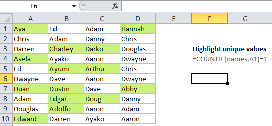
Formula

=COUNTIF(data,A1)=1

Explanation

Excel contains many built-in “presets” for highlighting values with conditional formatting, including a preset to highlight unique values. However, if you want more flexibility, you can highlight unique values with your own formula, as explained in this article.

If you want to highlight cells that contain unique values in a set of data, you can use a formula that returns TRUE when a value appears just once .

For example, if you have values in the cells A1:D10, and want to highlight cells with duplicate values, you can use this formula:

=COUNTIF($A$1:$D$10,A1)=1

Note: with conditional formatting, it’s important that the formula be entered relative to the “active cell” in the selection, which is assumed to be A1 in this case.

How this formula works

COUNTIF simply counts the number of times each value appears in the data range. By definition, each value must appear at least once, so when the count equals 1, the value is unique. When the count is 1, the formula returns TRUE and triggers the rule.

Conditional formatting is evaluated for each cell that is applied to. When you use a formula to apply conditional formatting, the formula is evaluated relative to the active cell in the selection at the time the rule is created. In this case, the range we are using in COUNTIF is locked with an absolute address, but A1 is fully relative. So, the rule is evaluated for each of the 40 cells in A1:D10, and A1 will be updated to a new address 40 times (once per cell) while $A$1:$D$10 remains unchanged.

Named ranges for a cleaner syntax

Another way to lock references is is to use named ranges, since named ranges are automatically absolute. For example, if you name the range A1:D10 “data”, you can rewrite the rule with a cleaner syntax like so:

=COUNTIF(data,A1)=1