
Skip to content
Free Excel Tutorials
  • Home
  • Excel For Beginners
  • Excel Intermediate
  • Advanced Excel For Experts

Data Analysis

  • How To Create Frequency Distribution in Excel
  • Calculate Conditional Percentile ‘IF’ in table in Excel
  • How to create dynamic reference table name in Excel
  • Conditional Formatting New Rule with Formulas in Excel
  • How to calculate current stock or inventory in Excel

References

  • How to use Excel MMULT Function
  • How to use Excel INDIRECT Function
  • Count rows that contain specific values in Excel
  • How to retrieve first match between two ranges in Excel
  • Find Closest Match in Excel Using INDEX, MATCH, ABS and MIN functions

Data Validations

  • How To Create Drop-down List in Excel
  • Excel Data validation specific characters only
  • Excel Data validation allow weekday only
  • Excel Data validation number multiple 100
  • Excel Data validation exists in list

Highlight duplicate columns in Excel

by

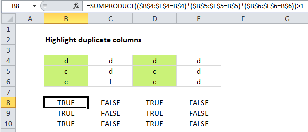
This tutorial shows how to  Highlight duplicate columns in Excel using the example below;

Formula

=SUMPRODUCT((row1=ref1)*(row2=ref2)*(row3=ref3))>1
Explanation

Excel contains a built-in preset for highlighting duplicate values with conditional formatting, but it only works at the cell level. If you want to find and highlight duplicate columns, you’ll need to use your own formula, as explained below.

To highlight duplicate columns, you can use a formula based on the SUMPRODUCT function.  In the example shown, the formula used to highlight duplicate columns is:

=SUMPRODUCT(($B$4:$E$4=B$4)*($B$5:$E$5=B$5)*($B$6:$E$6=B$6))>1

How this formula works

This approach uses SUMPRODUCT to count the occurrence of every value in the table, one row at a time. Only when the same value appears in the same location in all three rows is a count generated. For cell B4, the formula is solved like this:

=SUMPRODUCT(($B$4:$E$4=B$4)*($B$5:$E$5=B$5)*($B$6:$E$6=B$6))>1
=SUMPRODUCT(({1,1,1,1})*({1,0,1,0})*({1,0,1,0}))>1
=SUMPRODUCT({1,0,1,0})>1
=2>1
=TRUE

Note that row references are fully absolute, while cell references are mixed, with only the row locked.

With a helper row

If you don’t mind adding a helper row to your data, you can simplify the conditional formatting formula quite a bit. In a helper row, concatenate all values in the column. Then you can use COUNTIF on that one row to count values that appear more than once, and use the result to trigger conditional formatting in the entire column.

Post navigation

Previous Post:

COSH function: Description, Usage, Syntax, Examples and Explanation

Next Post:

Excel Data validation require unique number

Leave a Reply Cancel reply

Your email address will not be published. Required fields are marked *

Learn Basic Excel

Ribbon
Workbook
Worksheets
Format Cells
Find & Select
Sort & Filter
Templates
Print
Share
Protect
Keyboard Shortcuts

Categories

  • Charts
  • Data Analysis
  • Data Validation
  • Excel Functions
    • Cube Functions
    • Database Functions
    • Date and Time Functions
    • Engineering Functions
    • Financial Functions
    • Information Functions
    • Logical Functions
    • Lookup and Reference Functions
    • Math and Trig Functions
    • Statistical Functions
    • Text Functions
    • Web Functions
  • Excel VBA
  • Excel Video Tutorials
  • Formatting
  • Grouping
  • Others

Logical Functions

  • Nested IF function example in Excel
  • Invoice status with nested if in Excel
  • IF function: Description, Usage, Syntax, Examples and Explanation
  • How to use Excel AND Function
  • How to use IFS function in Excel

Date Time

  • How to calculate next day of week in Excel
  • Get days, hours, and minutes between dates in Excel
  • YEARFRAC function: Description, Usage, Syntax, Examples and Explanation
  • Get days between dates ignoring years in Excel
  • How to calculate Next working/business day in Excel

Grouping

  • Group times into 3 hour buckets in Excel
  • Calculate conditional mode with criteria in Excel
  • Map inputs to arbitrary values in Excel
  • How to randomly assign data to groups in Excel
  • Map text to numbers in Excel

General

  • Convert column number to letter in Excel
  • 44 Practical Excel IF function Examples
  • Cell References: Relative, Absolute and Mixed Referencing Examples
  • How to get original price from percentage discount in Excel
  • How to calculate profit margin percentage in Excel
© 2026 xlsoffice . All Right Reserved. | Teal Smiles | Abbreviations And Their Meaning