Count rows with multiple OR criteria in Excel

This tutorial shows how to Count rows with multiple OR criteria in Excel using the example below;

Formula

=SUMPRODUCT(--((criteria1)+(criteria2)>0))

Explanation

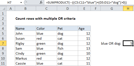
To count rows using multiple criteria across different columns – with OR logic – you can use the SUMPRODUCT function. In the example shown, the formula in H7 is:

=SUMPRODUCT(--((C5:C11="blue")+(D5:D11="dog")>0))

How this formula works

In the example shown, we want to count rows where the color is “blue”, OR the pet is “dog”.

The SUMPRODUCT function works with arrays natively so for the first criteria, we use:

(C5:C11="blue")

This returns an array of TRUE FALSE values like this:

{TRUE;FALSE;FALSE;TRUE;FALSE;FALSE;TRUE}

For the second criteria, we use:

(D5:D11="dog")

Which returns:

{TRUE;FALSE;TRUE;FALSE;TRUE;FALSE;FALSE}

These two arrays are then joined with addition (+), which automatically coerces the TRUE FALSE values to 1s and 0s to create an array like this:

{2;0;1;1;1;0;1}

We can’t simply add these values up with SUMPRODUCT because that would double count rows with both “blue” and “dog”. So, we use “>0” together with the double negative (–) to force all values to either 1 or zero:

--({2;0;1;1;1;0;1}>0)

Which presents this array to SUMPRODUCT:

{1;0;1;1;1;0;1}

SUMPRODUCT then returns the sum of all elements.

Other logical tests

The example shown tests for simple equality, but you can replace those statements with other logical tests as needed. For example, to count rows where cells in column A contain “red” OR cells in column B contain “blue”, you could use a formula like this:

=SUMPRODUCT(--(ISNUMBER(SEARCH("red",A1:A10))+ISNUMBER(SEARCH("blue",B1:B10))>0))