Calculate Weighted Average in Excel

To calculate a weighted average in Excel, simply use the SUMPRODUCT and the SUM function.

1. The AVERAGE function below calculates the normal average of three scores.

Suppose your teacher says, “The test counts twice as much as the quiz and the final exam counts three times as much as the quiz”.

2. Below you can find the corresponding weights of the scores.

The formula below calculates the weighted average of these scores.

Weighted Average	=	20 + 40 + 40 + 90 + 90 + 90
		6

=	370	=	61.67
	6

3. We can use the SUMPRODUCT function in Excel to calculate the number above the fraction line (370).

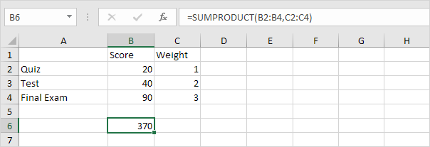
Note: the SUMPRODUCT function performs this calculation: (20 * 1) + (40 * 2) + (90 * 3) = 370.

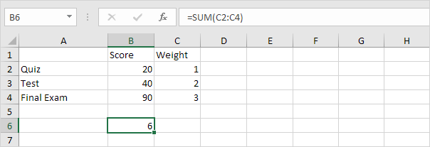
4. We can use the SUM function in Excel to calculate the number below the fraction line (6).

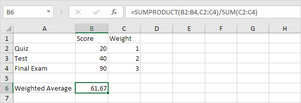
5. Use the functions at step 3 and step 4 to calculate the weighted average of these scores in Excel.