Win loss points calculation in Excel

This tutorial shows how to work Win loss points calculation in Excel using the example below;

To assign points based on win/loss/tie results for a team, you can use a simple VLOOKUP formula, or a nested IF formula, as explained below.

Formula

=VLOOKUP(result,points_table,2,0)

Explanation

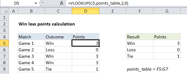
In the example shown, the formula in D5 is:

=VLOOKUP(C5,points_table,2,0)

How this formula works

This is a very simple application of the VLOOKUP function set for “exact match”:

• lookup value comes from C5
• table array is the named range “points_table” (F5:G7)
• column index is 2, since points are in column G
• range lookup is 0 (FALSE) to force exact match

Because we are using VLOOKUP in exact match mode, the points table does not need to be sorted in any particular way.

VLOOKUP is a nice solution in this case if you want to display the points table as a “key” for reference on the worksheet. If you don’t need to do this, see the nested IF version below.

Nested IF version

To calculate win/loss/tie points with the IF function, you can use a simple nested IF:

=IF(C5="Win",3,IF(C5="Loss",0,IF(C5="Tie",1)))