VLOOKUP with 2 lookup tables in Excel

To use VLOOKUP with a variable table array, you can use the IF function inside VLOOKUP to control which table is used.

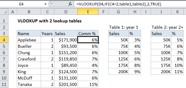
In the example shown the formula in cell E4 is:

=VLOOKUP(D5,IF(C4<2,table1,table2),2,TRUE)

This formula uses the number of years a salesperson has been with a company to determine which commission rate table to use.

How this formula works

Working from the inside out, the IF function in this formula, which is entered as the “table_array” argument in VLOOKUP, runs a logical test on the value in column C “Years”, which represents the number of years a salesperson has been with a company. If C5 is less than 2, then table1 is returned as the value if true. If C4 is greater than 2, table2 is returned as the value if false.

In other words, if years is less than 2, table1 is used as for table_array, and, if not, table2 is used as for table_array.

Alternate syntax

If the lookup tables require different processing rules, then you can wrap two VLOOKUP functions inside of an IF function like so:

=IF(test,VLOOKUP (value,table1,col,match),VLOOKUP (value,table2,col,match))

This allows you to customize the inputs to each VLOOKUP as needed.