Prevent invalid Product Codes or ID Numbers in Excel

This example teaches you how to use data validation to prevent users from entering incorrect product codes.

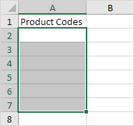
1. Select the range A2:A7.

2. On the Data tab, in the Data Tools group, click Data Validation.

3. In the Allow list, click Custom.

4. In the Formula box, enter the formula shown below and click OK.

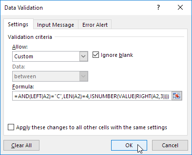
Explanation: this AND function has three arguments. LEFT(A2)=”C” forces the user to start with the letter C. LEN(A2)=4 forces the user to enter a string with a length of 4 characters. ISNUMBER(VALUE(RIGHT(A2,3))) forces the user to end with 3 numbers. RIGHT(A2,3) extracts the 3 rightmost characters from the text string. The VALUE function converts this text string to a number. ISNUMBER checks whether this value is a number. The AND Function returns TRUE if all conditions are true. Because we selected the range A2:A7 before we clicked on Data Validation, Excel automatically copies the formula to the other cells.

5. To check this, select cell A3 and click Data Validation.

As you can see, this cell also contains the correct formula.

6. Enter an incorrect product code.

Result. Excel shows an error alert.

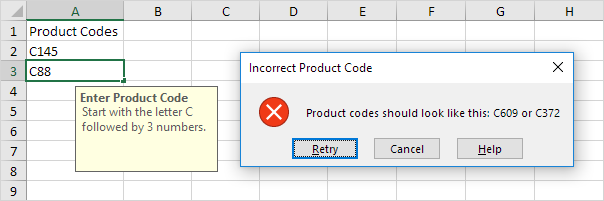
Note: to enter an input message and error alert message, go to the Input Message and Error Alert tab.