If cell is this OR that in Excel

This tutorial shows how to calculate If cell is this OR that in Excel using the example below;

Formula

=IF(OR(A1="this",A1="that"),"x","")

Explanation

If you want to do something specific when a cell equals this or that (i.e. is equal to X or Y, etc.) you can use the IF function in combination with the OR function to run a test, then take one action if the result is TRUE, and (optionally) do something else if the result of the test is FALSE.

If color is red or green, mark with “x”

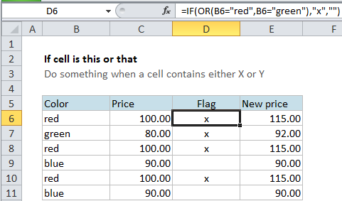
In the example shown, we simply want to “mark” or “flag” records where the color is either red OR green. In other words, we want to check cells in column B, and then take action when they contain the word “red” or the word “green”.

In D6, the formula were using is this:

=IF(OR(B6="red",B6="green"),"x","")

In this formula, the logical test is this bit:

OR(B6="red",B6="green")

This snippet will return TRUE if the value in B6 is either “red” OR “green” and FALSE if not.

Since we want to flag both red and green items, we need to take an action when the result of the test is TRUE. In this case, we do that by adding an “x” to column D. If the test is FALSE,  we simply add an empty string (“”). This causes an “x” to appear in column D when the value in column B is either “red” or “green” and nothing to appear if not.

Note: if we didn’t add the empty string when FALSE, the formula would actually display FALSE whenever the color is not red.

Increase price if color is red or green

If you need to do something more complex, just extend the formula.

For example, say you want to increase the price of red and green items only by 15%. In that case, you could use this formula in column E to calculate a new price:

=IF(OR(B6="red",B6="green"),C6*1.15,C6)

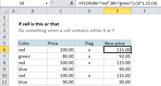
The test is the same as before, the action to take if TRUE is new.

If the result is TRUE, we multiply the original price by 1.15 (to increase by 15%). If the result of the test is FALSE, we simply output the original price.