Skip to content
Free Excel Tutorials
  • Home
  • Excel For Beginners
  • Excel Intermediate
  • Advanced Excel For Experts

Data Analysis

  • How to count table rows in Excel
  • Chart Axes in Excel
  • How to add Trendline to a chart in Excel
  • Get column index in Excel Table
  • Excel Bar Chart

References

  • How to get first row number in range in Excel
  • How to retrieve first match between two ranges in Excel
  • Count rows that contain specific values in Excel
  • How to use Excel INDIRECT Function
  • INDEX function: Description, Usage, Syntax, Examples and Explanation

Data Validations

  • Excel Data validation allow weekday only
  • Excel Data validation date in specific year
  • Prevent invalid data entering in specific cells
  • Excel Data validation must begin with
  • Excel Data validation don’t exceed total

Get last match cell contains in Excel

by

This tutorial shows how to Get last match cell contains in Excel using the example below;

Formula

=LOOKUP(2,1/SEARCH(things,A1),things)

Explanation

To check a cell for one of several things, and return the last match found in the list, you can use a formula based on the LOOKUP and SEARCH functions. In the case of multiple matches found, the formula will return the last match from the list of “things”.
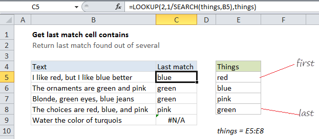
In the example shown, the formula in C5 is:

=LOOKUP(2,1/SEARCH(things,B5),things)

How this formula works

Context: you have a list of things in the named range “things” (E5:E8), and you want to check cells in column B to see if they contain these things. If so, you want to return the last item from”things” that was found.

In this formula, the SEARCH function is used to search cells in column B like this:

SEARCH(things,B5)

When SEARCH finds a match, it returns the position of the match in the cell being searched. When search can’t find a match, it returns the #VALUE error. Because we are giving SEARH more than one thing to look for, it will return more than one result. In the example shown, SEARCH returns an array of results like this:

{8;24;#VALUE!;#VALUE!}

This array is then used as a divisor for the number 1. The result is an array composed of errors and decimal values. The errors represent things not found, and the decimal values represent things found. In the example shown, the array looks like this:

{0.125;0.0416666666666667;#VALUE!;#VALUE!}

This array serves as the “lookup_vector” for the LOOKUP function. The lookup value is supplied as the number 2, and the result vector is the named range “things”. This is the clever part.

The formula is constructed in such a way so that the lookup vector will never contain a value larger than 1, while the the lookup value is 2. This means the lookup value will never be found. In this case, LOOKUP will match the last numeric value found in the array, which corresponds to the last “thing” found by SEARCH.

Finally, using the named range “things” supplied as the result vector, LOOKUP returns the last thing found.

With hard-coded values

Using a range like “things” makes it easy to modify the list of search terms (and add more search terms), but it’s not a requirement. You can also hard-code values directly into the formula like this:

=LOOKUP(2,1/SEARCH({"red","blue","green"},B5),{"red","blue","green"})

Post navigation

Previous Post:

COSH function: Description, Usage, Syntax, Examples and Explanation

Next Post:

Excel Data validation require unique number

Leave a Reply Cancel reply

Your email address will not be published. Required fields are marked *

Learn Basic Excel

Ribbon
Workbook
Worksheets
Format Cells
Find & Select
Sort & Filter
Templates
Print
Share
Protect
Keyboard Shortcuts

Categories

  • Charts
  • Data Analysis
  • Data Validation
  • Excel Functions
    • Cube Functions
    • Database Functions
    • Date and Time Functions
    • Engineering Functions
    • Financial Functions
    • Information Functions
    • Logical Functions
    • Lookup and Reference Functions
    • Math and Trig Functions
    • Statistical Functions
    • Text Functions
    • Web Functions
  • Excel VBA
  • Excel Video Tutorials
  • Formatting
  • Grouping
  • Others

Logical Functions

  • Nested IF function example in Excel
  • Return blank if in Excel
  • How to use Excel TRUE Function
  • Invoice status with nested if in Excel
  • IFNA function: Description, Usage, Syntax, Examples and Explanation

Date Time

  • DAYS360 function: Description, Usage, Syntax, Examples and Explanation
  • Add workdays to date custom weekends in Excel
  • How to calculate nth day of week in month in Excel
  • Get days between dates in Excel
  • Display Days until expiration date in Excel

Grouping

  • Group arbitrary text values in Excel
  • Group times into unequal buckets in Excel
  • Map text to numbers in Excel
  • If cell contains one of many things in Excel
  • Map inputs to arbitrary values in Excel

General

  • How to test a range for numbers in Excel
  • How to get random value from list or table in Excel
  • How to calculate decrease by percentage in Excel
  • Excel Operators
  • Subtotal by color in Excel
© 2025 xlsoffice . All Right Reserved. | Teal Smiles | Abbreviations And Their Meaning