Skip to content
Free Excel Tutorials
  • Home
  • Excel For Beginners
  • Excel Intermediate
  • Advanced Excel For Experts

Data Analysis

  • Data Series in Excel
  • How to sum a total in multiple Excel tables
  • Managing Conditional Formatting Rules in Excel
  • How to count table rows in Excel
  • Subtotal function in Excel

References

  • Approximate match with multiple criteria in Excel
  • How to create dynamic named range with OFFSET in Excel
  • Create hyperlink with VLOOKUP in Excel
  • Offset in Excel
  • Lookup entire row in Excel

Data Validations

  • Excel Data validation exists in list
  • Excel Data validation date in next 30 days
  • Excel Data validation unique values only
  • Excel Data validation require unique number
  • How To Create Drop-down List in Excel

Get information corresponding to max value in Excel

by

This tutorial shows how to Get information corresponding to max value in Excel using the example below;

Formula

=INDEX(range1,MATCH(MAX(range2),range2,0)

Explanation

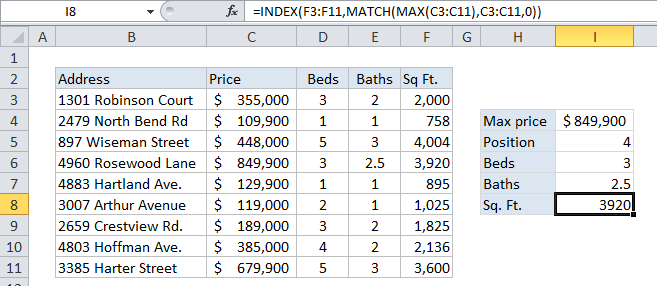
To lookup information related to the maximum value in a range, you can use a formula that combines the MAX, INDEX, and MATCH functions. In the example shown, the formula in I8 is:

=INDEX(F3:F11,MATCH(MAX(C3:C11),C3:C11,0))

Which returns the number 3920, representing the square footage (Sq. Ft.) of the most expensive property in the list.

How this formula works

The MAX function first extracts the maximum value from the range C3:C11.

In this case, that value is 849900.

This number is then supplied to the MATCH function as the lookup value. The lookup_array is the same range C3:C11, and the match_type is set to “exact” with 0.

Based on this information, the MATCH function locates and returns the relative position of the max value in the range, which is 4 in this case.

The number 4 is supplied to INDEX as “row number” along with the range F3:F11, supplied as the lookup array. INDEX then returns the value in the 4th position in F3:F11m which is 3924.

Note: in case of duplicates (i.e. two or more max values that are the same) this formula will return info for the first match, the default behavior of the MATCH function.

Post navigation

Previous Post:

How to use Excel CHOOSE Function

Next Post:

Customize Ribbon In Excel

Leave a Reply Cancel reply

Your email address will not be published. Required fields are marked *

Learn Basic Excel

Ribbon
Workbook
Worksheets
Format Cells
Find & Select
Sort & Filter
Templates
Print
Share
Protect
Keyboard Shortcuts

Categories

  • Charts
  • Data Analysis
  • Data Validation
  • Excel Functions
    • Cube Functions
    • Database Functions
    • Date and Time Functions
    • Engineering Functions
    • Financial Functions
    • Information Functions
    • Logical Functions
    • Lookup and Reference Functions
    • Math and Trig Functions
    • Statistical Functions
    • Text Functions
    • Web Functions
  • Excel VBA
  • Excel Video Tutorials
  • Formatting
  • Grouping
  • Others

Logical Functions

  • How to use Excel TRUE Function
  • Check multiple cells are equal in Excel
  • Return blank if in Excel
  • Not Equal To ‘<>‘ operator in Excel
  • How to use IFS function in Excel

Date Time

  • Add business days to date in Excel
  • NETWORKDAYS.INTL function: Description, Usage, Syntax, Examples and Explanation
  • Display Date is workday in Excel
  • How to get year from date in Excel
  • EDATE function: Description, Usage, Syntax, Examples and Explanation

Grouping

  • Calculate conditional mode with criteria in Excel
  • If cell contains one of many things in Excel
  • Group numbers with VLOOKUP in Excel
  • Categorize text with keywords in Excel
  • Group times into unequal buckets in Excel

General

  • Basic text sort formula in Excel
  • Share Excel data with Word documents
  • Find Most Frequently Occurring Word in Excel Worksheet
  • How to calculate decrease by percentage in Excel
  • Convert column number to letter in Excel
© 2026 xlsoffice . All Right Reserved. | Teal Smiles | Abbreviations And Their Meaning