How to extract text between parentheses in Excel

To extract text between parentheses, braces, brackets, etc. you can use a formula based on the MID function, with help from SEARCH function.

Formula

=MID(text,SEARCH("(",text)+1,SEARCH(")",
text)-SEARCH("(",text)-1)

Explanation

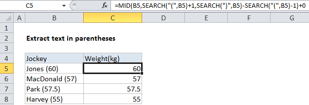
In the example shown, the formula in C5 is:

=MID(B5,SEARCH("(",B5)+1,SEARCH
(")",B5)-SEARCH("(",B5)-1)+0

How this formula works

The foundation of this formula is the MID function, which extracts a specific number of characters from text, starting at a specific location. To figure out where to start extracting text, we use this expression:

SEARCH("(",B5)+1

This locates the left parentheses and adds 1 to get the position of the first character inside the parentheses. To figure out how many characters to extract, we use this expression:

SEARCH(")",B5)-SEARCH("(",B5)-1

This locates the second parentheses in the text, and subtracts the position of the first parentheses (less one) to get the total number of characters that need to be extracted. With this information, MID extracts just the text inside the parentheses.

Finally, because we want a number as the final result in this particular example, we add zero to text value returned by MID:

+0

This math operation causes Excel to coerce text values to numbers. If you don’t need or want a number at the end, this step is not required.